lonboard

Render tens or hundreds of thousands of GPU-accelerated map points, with pan/zoom/click/box-select wired back into Shiny as reactive inputs.

lonboard is a GPU-accelerated map widget from Development Seed, built on deck.gl and GeoArrow. Where most Python map widgets serialize GeoJSON and render on the CPU, lonboard moves Arrow-columnar geometry straight to the browser and draws it with WebGL – so a scatterplot of a few hundred thousand points pans and zooms as smoothly as a few hundred. It speaks GeoPandas, GeoArrow tables, and raw Arrow arrays natively, and ships a small set of purpose-built layers (scatter, path, polygon, arc, column, heatmap, point cloud, trips, H3, and a WebGL globe) rather than a general-purpose rendering pipeline.

@render_lonboard accepts a lonboard.Map, a layer (or list of layers), or anything lonboard.viz() understands – most commonly a GeoPandas GeoDataFrame or a GeoArrow-compatible Arrow table. It applies shinywidgets’ usual layout defaults (the map fills its container unless you give it an explicit pixel height) and gives every rendered map five reactive accessors – view_state(), selected(), selected_rows(), selected_bounds(), and clicked() – that turn pan, pick, box select, and click into values you read like input.x(). Those accessors are what make lonboard a genuine input, not just an output: a map can drive a chart, a table, or another map, the same way a slider drives a plot.

Reach for lonboard when the story is scale (tens of thousands of points or more) or GPU-native styling (data-driven color/radius via apply_continuous_cmap, extrusion, a WebGL globe). For tile-based basemaps with a more traditional Leaflet-style API and drawing tools, see ipyleaflet or leafmap; for vector-tile styling with a Mapbox GL / MapLibre style spec, see maplibre; for one-line “point in, clustered dashboard out” exploration, see keplergl.

hero

Installation

pip install 'shinywidgets[lonboard]'

This installs lonboard itself. GeoDataFrame input additionally needs geopandas and pyarrow (lonboard converts via geopandas_to_geoarrow); the examples below also use matplotlib for color ramps.

Quick start

A GeoDataFrame returned from a @render_lonboard function is converted with lonboard.viz(), which picks a layer type (ScatterplotLayer for points) and fits the initial view to the data – no Map or layer construction required.

examples/01_quickstart.py15 lines

import geopandas as gpd
from shiny.express import ui
from shinywidgets import render_lonboard

ui.page_opts(fillable=True)

# ~240 populated places from Natural Earth (110m scale), with longitude/
# latitude and population columns.
CITIES_URL = "https://raw.githubusercontent.com/nvkelso/natural-earth-vector/master/geojson/ne_110m_populated_places.geojson"


@render_lonboard
def map():
    cities = gpd.read_file(CITIES_URL)
    return cities  # lonboard.viz() picks a ScatterplotLayer and fits the view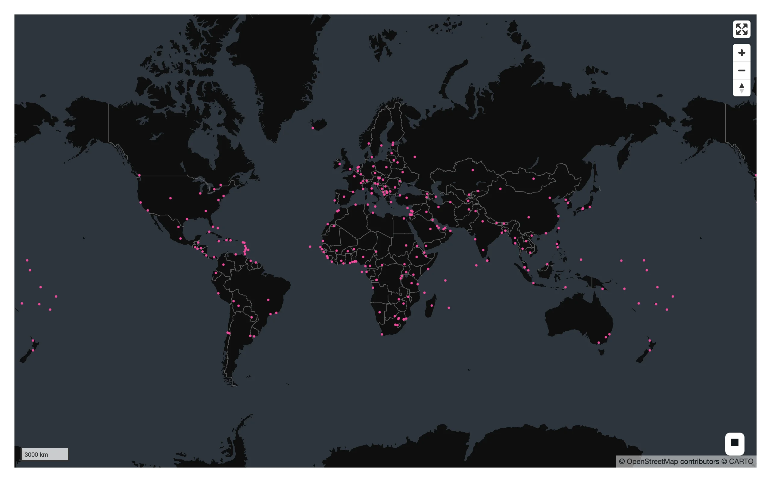

quickstart

What you can build

Choropleths with apply_continuous_cmap

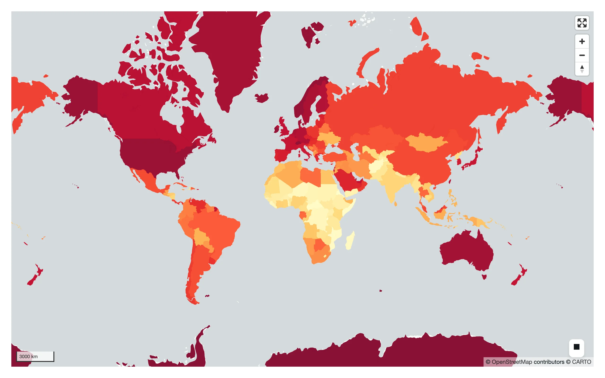
lonboard’s apply_continuous_cmap() turns a 0-1 array into per-row RGB(A) in one call, using any matplotlib colormap (or a palettable Palette). Pass the result straight to a layer’s get_fill_color.

examples/02_choropleth.py23 lines

import geopandas as gpd
import matplotlib.pyplot as plt
from lonboard import PolygonLayer
from lonboard.colormap import apply_continuous_cmap
from shiny.express import ui
from shinywidgets import render_lonboard

ui.page_opts(fillable=True)

COUNTRIES_URL = "https://raw.githubusercontent.com/nvkelso/natural-earth-vector/master/geojson/ne_110m_admin_0_countries.geojson"


@render_lonboard
def map():
    countries = gpd.read_file(COUNTRIES_URL)
    countries = countries[countries.GDP_MD > 0].copy()
    gdp_per_capita = countries.GDP_MD * 1e6 / countries.POP_EST
    # apply_continuous_cmap() takes values in [0, 1] and any matplotlib
    # colormap (or a palettable Palette), returning one uint8 RGB row per value
    colors = apply_continuous_cmap(gdp_per_capita.rank(pct=True), plt.get_cmap("YlOrRd"))
    return PolygonLayer.from_geopandas(
        countries, get_fill_color=colors, get_line_color=[80, 80, 80], opacity=0.85
    )

choropleth

Arcs, from plain arrays

Not every layer takes geometry. ArcLayer has no geometry column of its own – give it a table for the row count and plain float64 arrays for get_source_position/get_target_position. Because there’s no geometry, lonboard can’t auto-fit the view, so set one explicitly.

examples/03_arcs.py36 lines

import geopandas as gpd
import numpy as np
import pyarrow as pa
from lonboard import ArcLayer, Map
from lonboard.view_state import MapViewState
from shiny.express import ui
from shinywidgets import render_lonboard

ui.page_opts(fillable=True)

CITIES_URL = "https://raw.githubusercontent.com/nvkelso/natural-earth-vector/master/geojson/ne_110m_populated_places.geojson"
HUB = "London"
DESTINATIONS = ["New York", "Dubai", "Singapore", "Johannesburg", "Sydney", "Lima"]


@render_lonboard
def map():
    cities = gpd.read_file(CITIES_URL).set_index("NAME")
    hub_lon, hub_lat = cities.loc[HUB, ["LONGITUDE", "LATITUDE"]]
    dest = cities.loc[DESTINATIONS]
    n = len(dest)

    # ArcLayer has no geometry column of its own: pass source/target
    # coordinates as plain float64 arrays, with a dummy table for the row
    # count. Without geometry, lonboard can't auto-fit the view, so set one.
    layer = ArcLayer(
        table=pa.table({"name": dest.index.tolist()}),
        get_source_position=np.column_stack(
            [np.full(n, hub_lon), np.full(n, hub_lat)]
        ),
        get_target_position=dest[["LONGITUDE", "LATITUDE"]].to_numpy(dtype="float64"),
        get_source_color=[0, 200, 255],
        get_target_color=[255, 80, 80],
        get_width=3,
    )
    return Map(layer, view_state=MapViewState(longitude=10, latitude=20, zoom=0.8))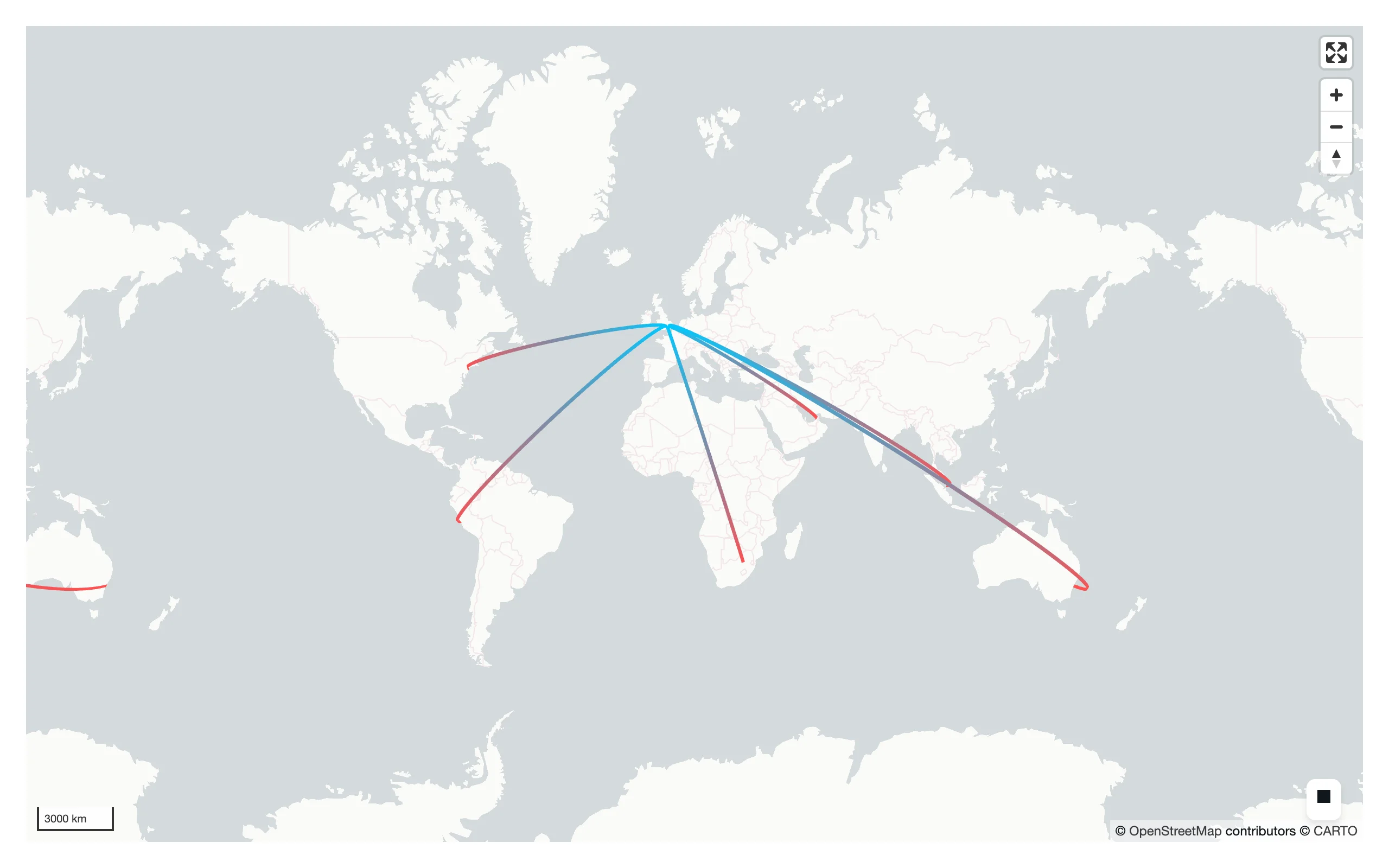

arcs

GeoArrow tables, no GeoPandas required

lonboard’s native format is GeoArrow. For data that’s already Arrow – a GeoParquet file, a DuckDB spatial query, a geoarrow-rust pipeline – you can build a layer directly from an Arrow table and skip GeoPandas/shapely entirely.

examples/04_geoarrow.py22 lines

import geoarrow.rust.core as gr
import numpy as np
from arro3.core import Table
from lonboard import ScatterplotLayer
from shiny.express import ui
from shinywidgets import render_lonboard

ui.page_opts(fillable=True)


# lonboard's native format is GeoArrow, not just GeoDataFrame: here a table is
# built directly from a GeoArrow point array, with no geopandas/shapely
# involved at all. This is the fastest path for data that's already Arrow
# (e.g., read from a GeoParquet file or a DuckDB spatial query).
@render_lonboard
def map():
    rng = np.random.default_rng(0)
    lon = rng.uniform(-74.05, -73.95, 2000)
    lat = rng.uniform(40.68, 40.78, 2000)
    points = gr.points((lon, lat), crs="EPSG:4326")
    table = Table.from_arrays([points], names=["geometry"])
    return ScatterplotLayer(table=table, get_fill_color=[0, 150, 255], radius_min_pixels=2)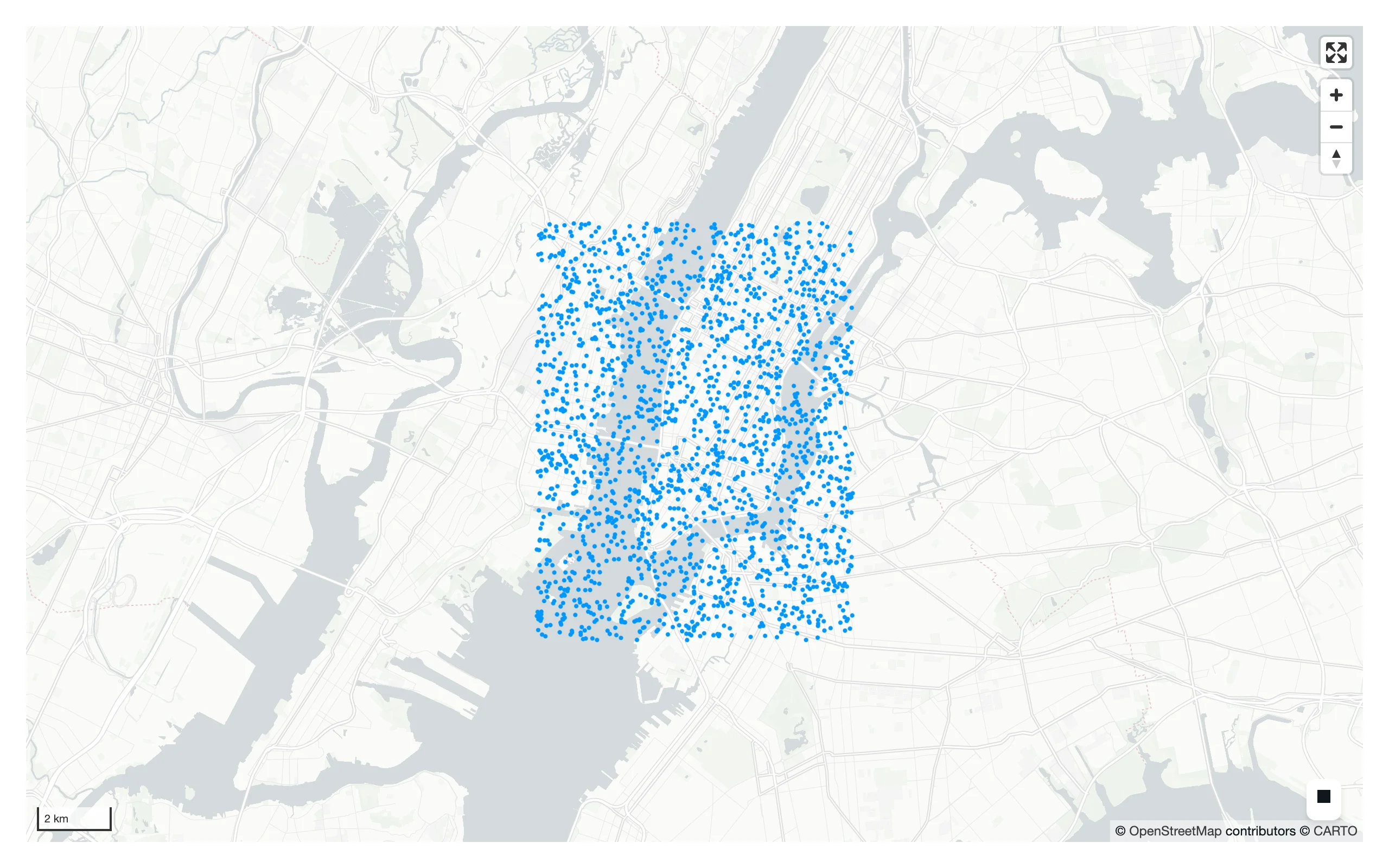

geoarrow

Multiple layers on one map

A Map takes a list of layers, drawn in order (last on top). Combine a polygon basemap layer with a point layer the same way you’d layer traces in a plotting library.

examples/05_multilayer.py28 lines

import geopandas as gpd
from lonboard import Map, PolygonLayer, ScatterplotLayer
from lonboard.basemap import CartoStyle, MaplibreBasemap
from shiny.express import ui
from shinywidgets import render_lonboard

ui.page_opts(fillable=True)

COUNTRIES_URL = "https://raw.githubusercontent.com/nvkelso/natural-earth-vector/master/geojson/ne_110m_admin_0_countries.geojson"
CITIES_URL = "https://raw.githubusercontent.com/nvkelso/natural-earth-vector/master/geojson/ne_110m_populated_places.geojson"


@render_lonboard
def map():
    countries = PolygonLayer.from_geopandas(
        gpd.read_file(COUNTRIES_URL),
        get_fill_color=[40, 40, 40],
        get_line_color=[90, 90, 90],
        opacity=0.6,
    )
    cities = ScatterplotLayer.from_geopandas(
        gpd.read_file(CITIES_URL),
        get_fill_color=[255, 210, 0],
        radius_min_pixels=2,
        pickable=True,
    )
    # A Map holds a list of layers; order determines draw order (last on top)
    return Map([countries, cities], basemap=MaplibreBasemap(style=CartoStyle.DarkMatter))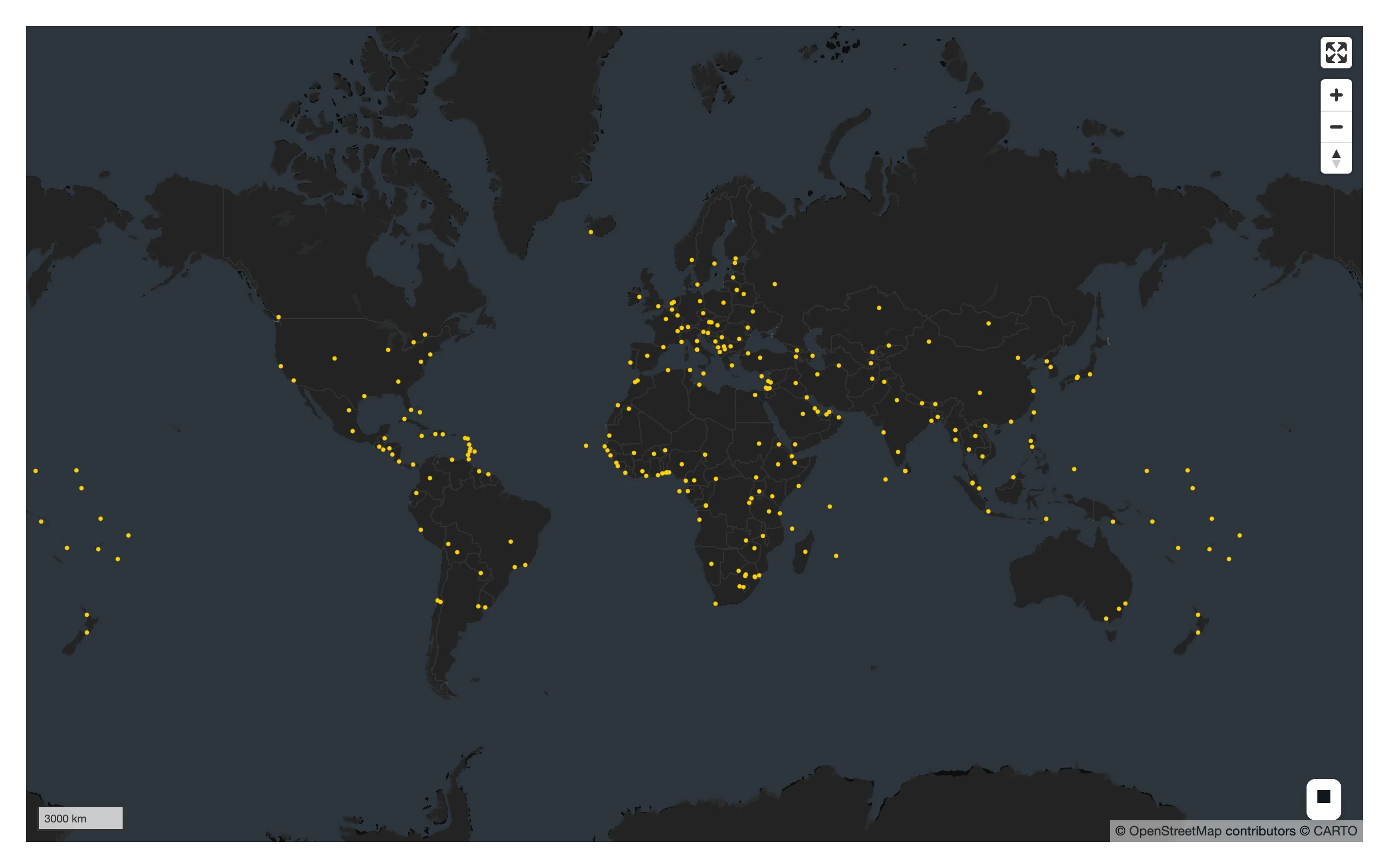

multilayer

A WebGL globe

Swapping view=GlobeView() (plus an interleaved basemap) turns the same layer into a rotatable WebGL globe – no other code changes.

examples/06_globe.py20 lines

import geopandas as gpd
from lonboard import Map, ScatterplotLayer
from lonboard._map import GlobeView
from lonboard.basemap import MaplibreBasemap
from shiny.express import ui
from shinywidgets import render_lonboard

ui.page_opts(fillable=True)

CITIES_URL = "https://raw.githubusercontent.com/nvkelso/natural-earth-vector/master/geojson/ne_110m_populated_places.geojson"


@render_lonboard
def map():
    cities = ScatterplotLayer.from_geopandas(
        gpd.read_file(CITIES_URL), get_fill_color=[255, 140, 0], radius_min_pixels=3
    )
    # Same layer, different view: GlobeView needs an interleaved basemap, and
    # lonboard raises a clear error if you forget it.
    return Map(cities, view=GlobeView(), basemap=MaplibreBasemap(mode="interleaved"))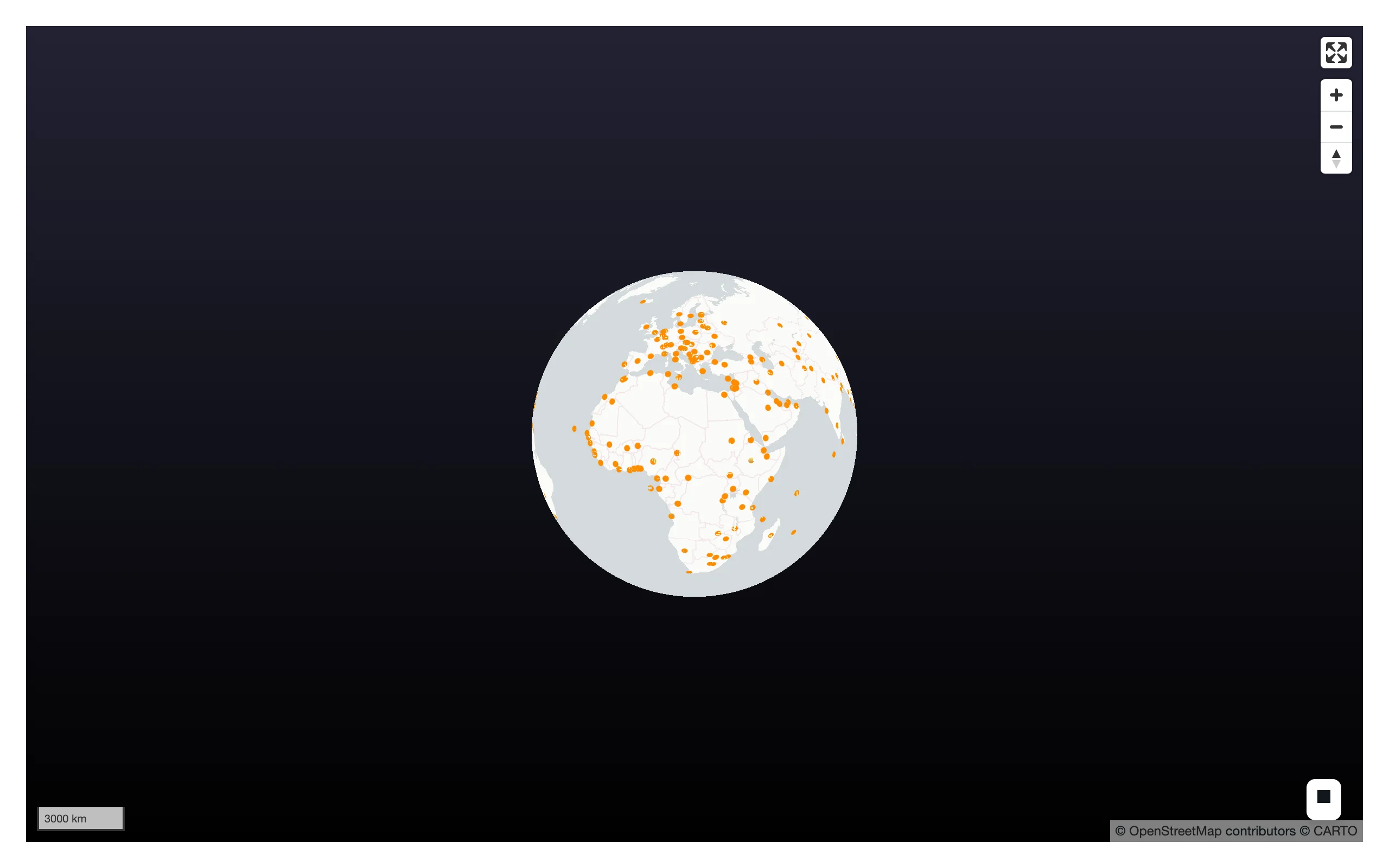

globe

Note: GlobeView is importable only from the private lonboard._map module today; there’s no public top-level export. See Gotchas for a real limitation this view has with the accessors below.

Reacting to user interaction

Accessor reference

Every accessor attaches the moment the map renders and records what the user does whether or not anything has read it yet – there’s no warm-up read to remember, and a pick, box selection, or click that happens before the first read still shows up in it.

Accessor	Returns	Before any interaction	Across re-render	Default rate policy
view_state()	MapViewState / GlobeViewState (lng/lat order: longitude, latitude, zoom, pitch, bearing)	Seeded (computed from the layers)	Re-seeded from the new map	Debounced, 250 ms
selected()	Optional[int], a positional row index	None	Re-seeded (a freshly built map starts with no pick)	None
selected_rows(df=None)	the picked row of df (default: a frame rebuilt from the pickable layer’s own data), in df’s own type	empty frame	derived from selected()	None
selected_bounds()	Optional[(minx, miny, maxx, maxy)], i.e. (west, south, east, north)	None	Re-seeded	None
clicked()	Optional[(lng, lat)]	None	Kept until the user clicks the new map	None

view_state() and selected()/selected_bounds() describe the map’s own state, so each re-render starts over from the new map’s state – a fresh map has no pick or selection, so those two are typically None again right after a re-render (immutable widget), while view_state() always has a value (computed from the new map’s layers). clicked() is different: a click is something the user did, not something the map owns, so it survives a re-render and keeps reporting the previous click until the user clicks the new map.

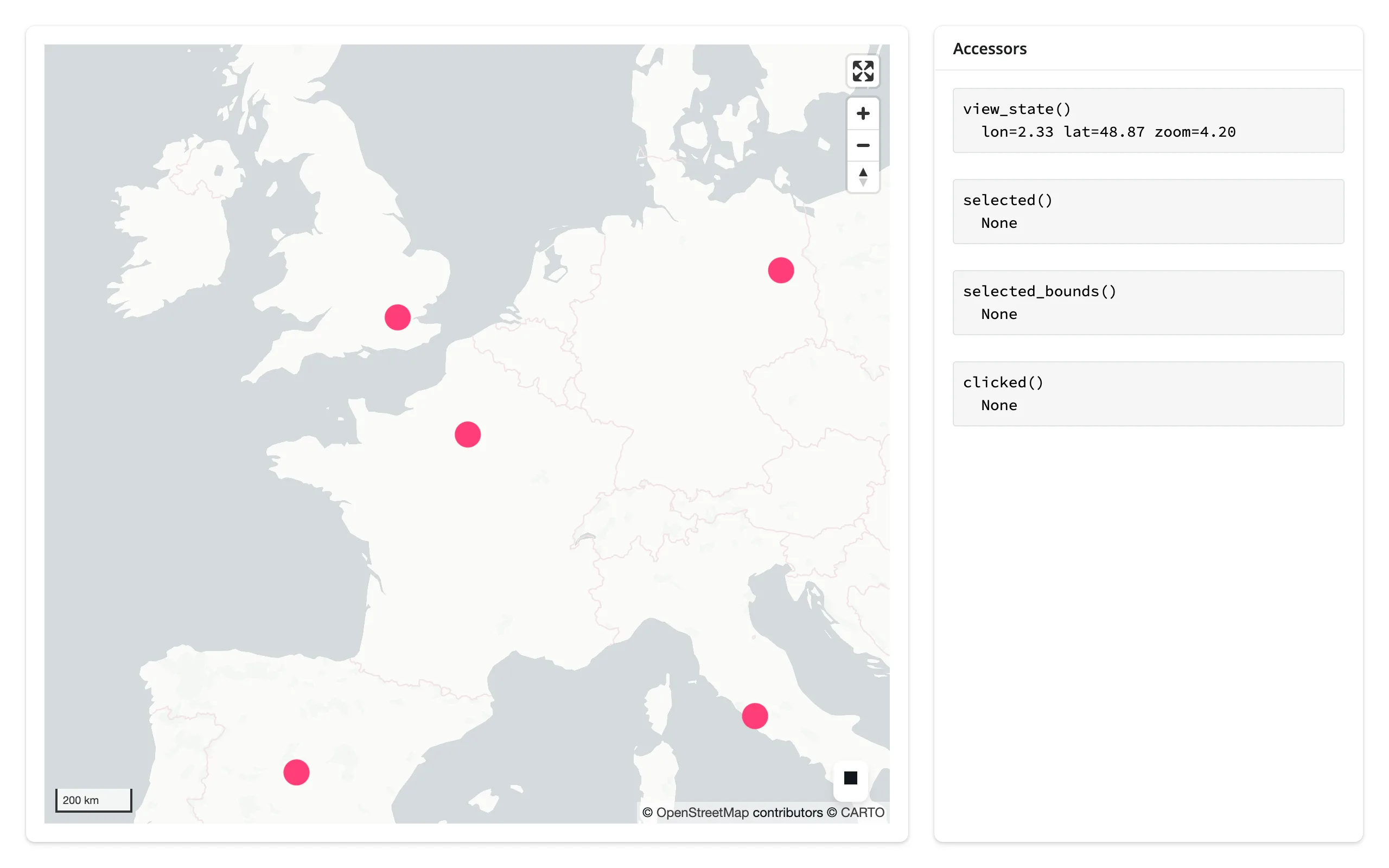
The four gesture accessors are exercised together below – pan the map, click a city, and drag a box with the Select BBox tool – rendered as raw values so you can see exactly what each one returns.

examples/07_accessors.py48 lines

import geopandas as gpd
from lonboard import Map, ScatterplotLayer
from lonboard.view_state import MapViewState
from shiny.express import render, ui
from shinywidgets import render_lonboard

ui.page_opts(fillable=True)

CITIES_URL = "https://raw.githubusercontent.com/nvkelso/natural-earth-vector/master/geojson/ne_110m_populated_places.geojson"
FOCUS = ["Paris", "London", "Berlin", "Madrid", "Rome"]

with ui.layout_columns(col_widths=[8, 4]):
    with ui.card(full_screen=True):

        @render_lonboard
        def map():
            cities = gpd.read_file(CITIES_URL)
            cities = cities[cities.NAME.isin(FOCUS)].reset_index(drop=True)
            layer = ScatterplotLayer.from_geopandas(
                cities, get_fill_color=[255, 60, 120], radius_min_pixels=12, pickable=True
            )
            return Map(
                layer,
                view_state=MapViewState(longitude=2.33, latitude=48.87, zoom=4.2),
                # Keep the canvas size stable; the "Accessors" card already
                # shows feature detail via selected()
                show_side_panel=False,
            )

    with ui.card():
        ui.card_header("Accessors")

        @render.code
        def view_state():
            vs = map.view_state()
            return f"view_state()\n  lon={vs.longitude:.2f} lat={vs.latitude:.2f} zoom={vs.zoom:.2f}"

        @render.code
        def selected():
            return f"selected()\n  {map.selected()}"

        @render.code
        def selected_bounds():
            return f"selected_bounds()\n  {map.selected_bounds()}"

        @render.code
        def clicked():
            return f"clicked()\n  {map.clicked()}"

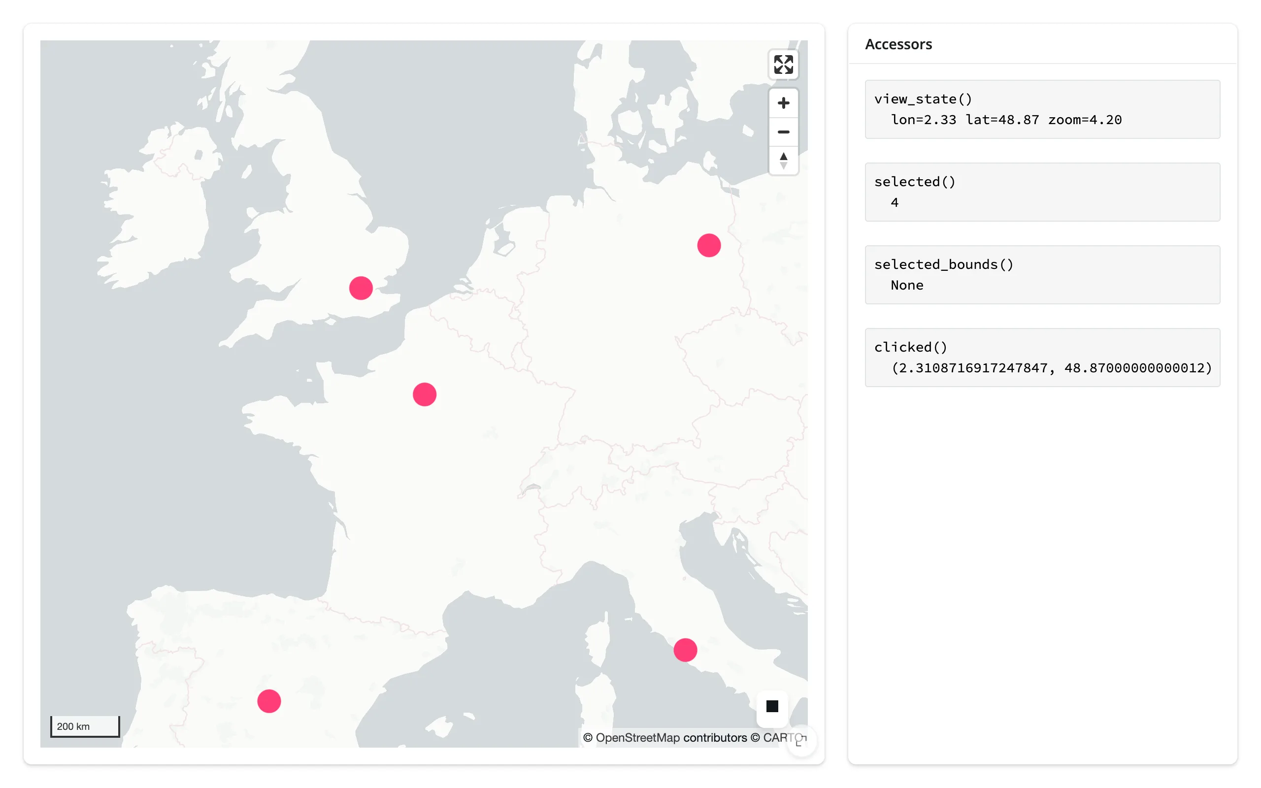
Before any interaction, view_state() is already populated (computed from the layer’s bounds); the other three are None:

accessors before

After panning, clicking Paris, and drawing a box over Western Europe, all four report their values – note clicked() and selected_bounds() are in (lng, lat) order, the opposite of ipyleaflet’s [lat, lng]:

accessors after

view_state()

Available immediately (it’s computed from the layer bounds at construction, not only after a gesture). The browser reports continuously through a pan, zoom, or rotate – every frame of the gesture – so this accessor debounces its publication to Python by 250 ms by default; each new report during an active gesture re-arms the debounce, so view_state() settles once the gesture pauses rather than updating on every frame. Override the window (or switch to "throttle") with render_lonboard’s rate_policy/rate_delay kwargs – see Rate limiting. The map itself is immutable per render, so a re-render always starts fresh from the new map’s own computed view state – view_state() is never None once rendered.

selected()

The positional index of the most recently picked row, across all pickable layers on the map – it can’t tell you which layer fired. When what you want is the picked row rather than its position, that’s selected_rows() below. Picking the same row of the same layer twice in a row doesn’t re-fire, and clicking empty space doesn’t clear it. A layer only reports picks when pickable=True (the default). Re-seeded on every re-render: a freshly built map starts with no pick, so selected() goes back to None until the new map reports one (the exception is a map that outlives its render, e.g. a shared_lifetime() map, which can carry a retained pick forward). With several pickable layers, read each layer’s own selected_index trait directly instead – see Beyond the accessors below.

selected_rows()

The picked row of a data frame – what selected() means when what you want is the row itself, for a detail card, a table, or a download. map.selected_rows() with no argument rebuilds the frame from the pickable layer’s own data (geopandas.GeoDataFrame.from_arrow(layer.table)), which keeps the layer’s rows and columns but not your original frame’s index: the result gets a fresh RangeIndex. Pass a frame explicitly – map.selected_rows(gdf) – when you need the original frame (or it isn’t a GeoDataFrame); any frame type works (pandas in, pandas out; polars in, polars out). It’s an empty frame while nothing is picked, so it can also be passed straight to @render.data_frame.

Two caveats:

• The default needs exactly one pickable layer and geopandas. Every lonboard layer can hold a pick, so a map with several layers (a choropleth under a city scatter, say) has no way to say which layer a pick came from – the default raises, and you pass df= for the layer you mean (or read each layer’s pick yourself, as in Beyond the accessors). The default also needs geopandas installed to rebuild the frame (it’s an optional dependency, not part of the shinywidgets[lonboard] extra); without it you get a clear ImportError, and df= works regardless.
• The match is positional (df.iloc[map.selected()]), so after a re-render or in-place data replacement (layer.table = ... on a long-lived map), a retained position can point at a different row – carry an ID column and look rows up by it when the data can change.

selected_bounds()

The bounding box from lonboard’s built-in Select BBox control, as (minx, miny, maxx, maxy) – west, south, east, north. The gesture is click, then click again at the opposite corner, not a drag; the button is always present in the map’s default controls. None until the first completed selection in this render, and re-seeded to None on every re-render – a freshly built map has no selection of its own. Setting selected_bounds from Python does not draw the overlay rectangle (the trait and the overlay rendering aren’t wired together upstream), so don’t try to seed a selection that way.

clicked()

The (lng, lat) of the most recent click anywhere on the map – including open ocean, unlike selected(), which only fires on a pickable feature. clicked() attaches the moment the map renders, whether or not anything has read it yet, so a click that happens before the first read still shows up in it. Clicking the same spot twice doesn’t re-fire. Unlike the other three accessors, a re-render doesn’t reset it: clicked() keeps reporting the previous click until the user clicks the new map (verified by clicking, forcing a re-render, and confirming the value survives – see NOTES.md).

Beyond the accessors: reactive_read

selected() tells you that something was picked, but not which layer, when a map has several pickable layers. For that, skip the accessor and reactive_read() each layer’s own selected_index trait directly – a layer is a child widget, not the rendered map itself, so there’s no .read() for it; reactive_read() is the tool for any widget that isn’t an output’s own .widget:

examples/08_reactive_read_layer.py56 lines

import geopandas as gpd
from lonboard import Map, ScatterplotLayer
from lonboard.view_state import MapViewState
from shiny.express import render, ui
from shinywidgets import reactive_read, render_lonboard

ui.page_opts(fillable=True)

CITIES_URL = "https://raw.githubusercontent.com/nvkelso/natural-earth-vector/master/geojson/ne_110m_populated_places.geojson"

# map.selected() reports "whichever pickable layer was clicked most
# recently" -- it can't tell the two apart. With several pickable layers,
# read each layer's own `selected_index` trait instead.
CAPITALS = ["Paris", "Madrid", "Rome"]
OTHERS = ["Brussels", "Luxembourg", "Geneva", "Bern", "Andorra"]

with ui.layout_columns(col_widths=[8, 4]):
    with ui.card(full_screen=True):

        @render_lonboard
        def map():
            cities = gpd.read_file(CITIES_URL).set_index("NAME")
            capitals = ScatterplotLayer.from_geopandas(
                cities.loc[CAPITALS].reset_index(),
                get_fill_color=[255, 60, 120],
                radius_min_pixels=10,
                pickable=True,
            )
            others = ScatterplotLayer.from_geopandas(
                cities.loc[OTHERS].reset_index(),
                get_fill_color=[80, 160, 255],
                radius_min_pixels=7,
                pickable=True,
            )
            return Map(
                [capitals, others],
                view_state=MapViewState(longitude=2.33, latitude=48.87, zoom=4.5),
                show_side_panel=False,
            )

    with ui.card():
        ui.card_header("Per-layer picks")

        @render.code
        def capital_pick():
            layer = map.widget.layers[0] if map.widget else None
            index = reactive_read(layer, "selected_index") if layer else None
            name = CAPITALS[index] if index is not None else None
            return f"capitals layer: {name}"

        @render.code
        def other_pick():
            layer = map.widget.layers[1] if map.widget else None
            index = reactive_read(layer, "selected_index") if layer else None
            name = OTHERS[index] if index is not None else None
            return f"others layer: {name}"

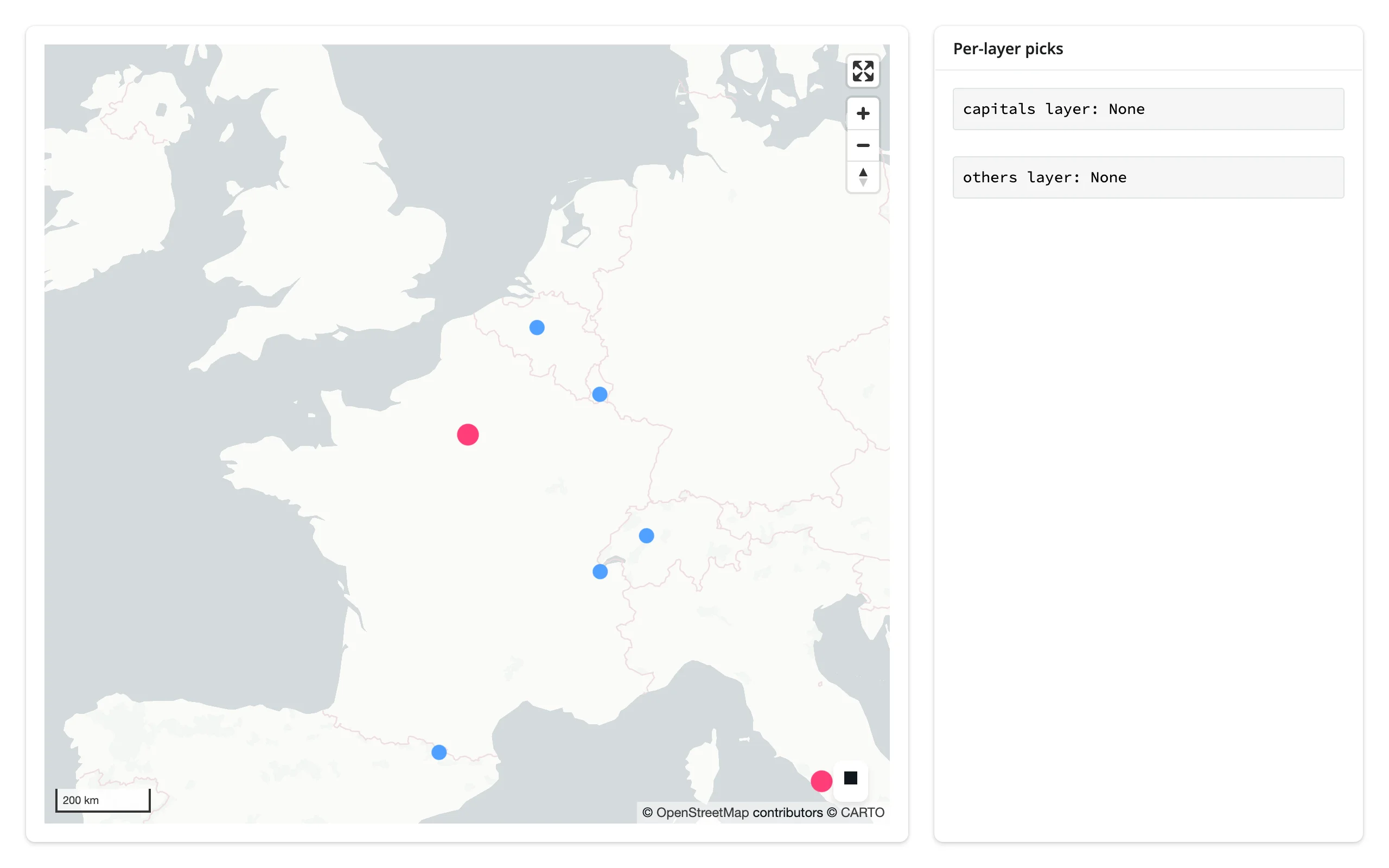
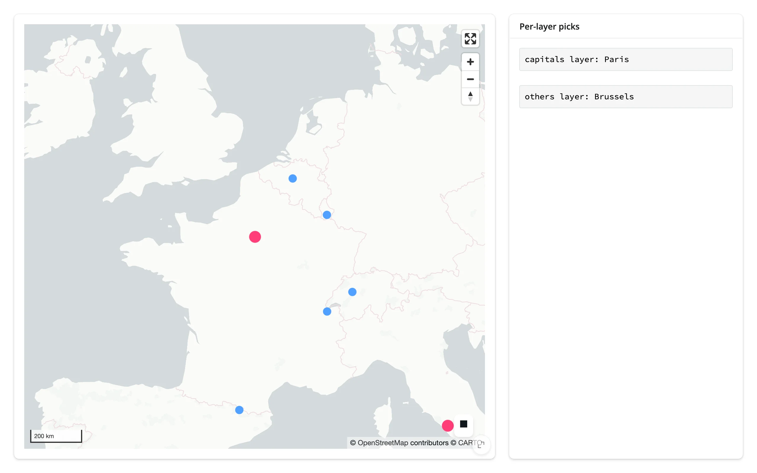
Picking a point from each layer updates its own readout independently:

Rate limiting

view_state() is the only accessor with a default rate policy – debounced 250 ms (see view_state() above). render_lonboard’s rate_policy/rate_delay kwargs adjust that default (and rate-limit reactive_read()/.read() on the map’s other traits); they have no effect on selected(), selected_bounds(), or clicked() (or selected_rows(), which follows selected()), since none of those declares a default policy of its own (verified directly: constructing render_lonboard(rate_policy="throttle", rate_delay=1.0) and inspecting its internal accessor slots shows a limiter only on view_state’s).

Pass rate_delay=0 to remove the debounce – every tick the browser reports publishes right away, useful when you want view_state() to drive something with no lag and can afford the extra re-renders downstream. map.read("view_state") and map.view_state() are the same read either way: "view_state" is a declared accessor name, so read() just calls the accessor.

examples/15_rate_limiting.py27 lines

import geopandas as gpd
from lonboard import ScatterplotLayer
from shiny.express import render, ui
from shinywidgets import render_lonboard

ui.page_opts(fillable=True)

CITIES_URL = "https://raw.githubusercontent.com/nvkelso/natural-earth-vector/master/geojson/ne_110m_populated_places.geojson"


# view_state() debounces by default (0.25 s). render_lonboard's rate_policy/
# rate_delay kwargs now adjust that default too, not just reactive_read() on
# the map's other traits: rate_delay=0 below removes the debounce entirely, so
# every tick the browser reports publishes right away.
@render_lonboard(rate_delay=0)
def map():
    cities = gpd.read_file(CITIES_URL)
    return ScatterplotLayer.from_geopandas(cities, get_fill_color=[255, 60, 120], radius_min_pixels=4)


@render.code
def coords():
    vs = map.view_state()
    # map.read("view_state") is the same read -- "view_state" is a declared
    # accessor name, so read() just calls the accessor method
    agree = map.read("view_state") == vs
    return f"lon={vs.longitude:.4f} lat={vs.latitude:.4f} zoom={vs.zoom:.2f}\nmap.read('view_state') agrees: {agree}"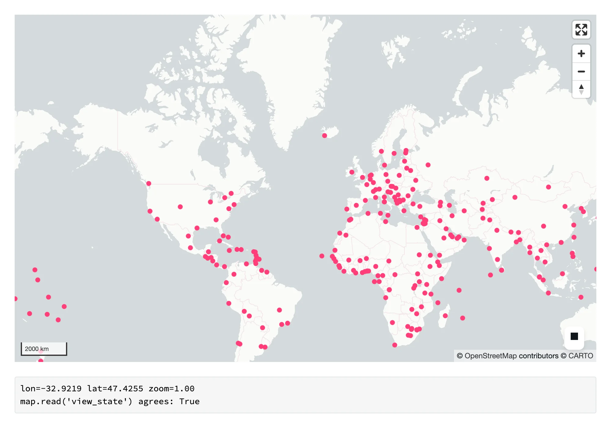

rate limiting

Updating the widget from Python

Two different Python-side actions look similar but do very different things to the browser:

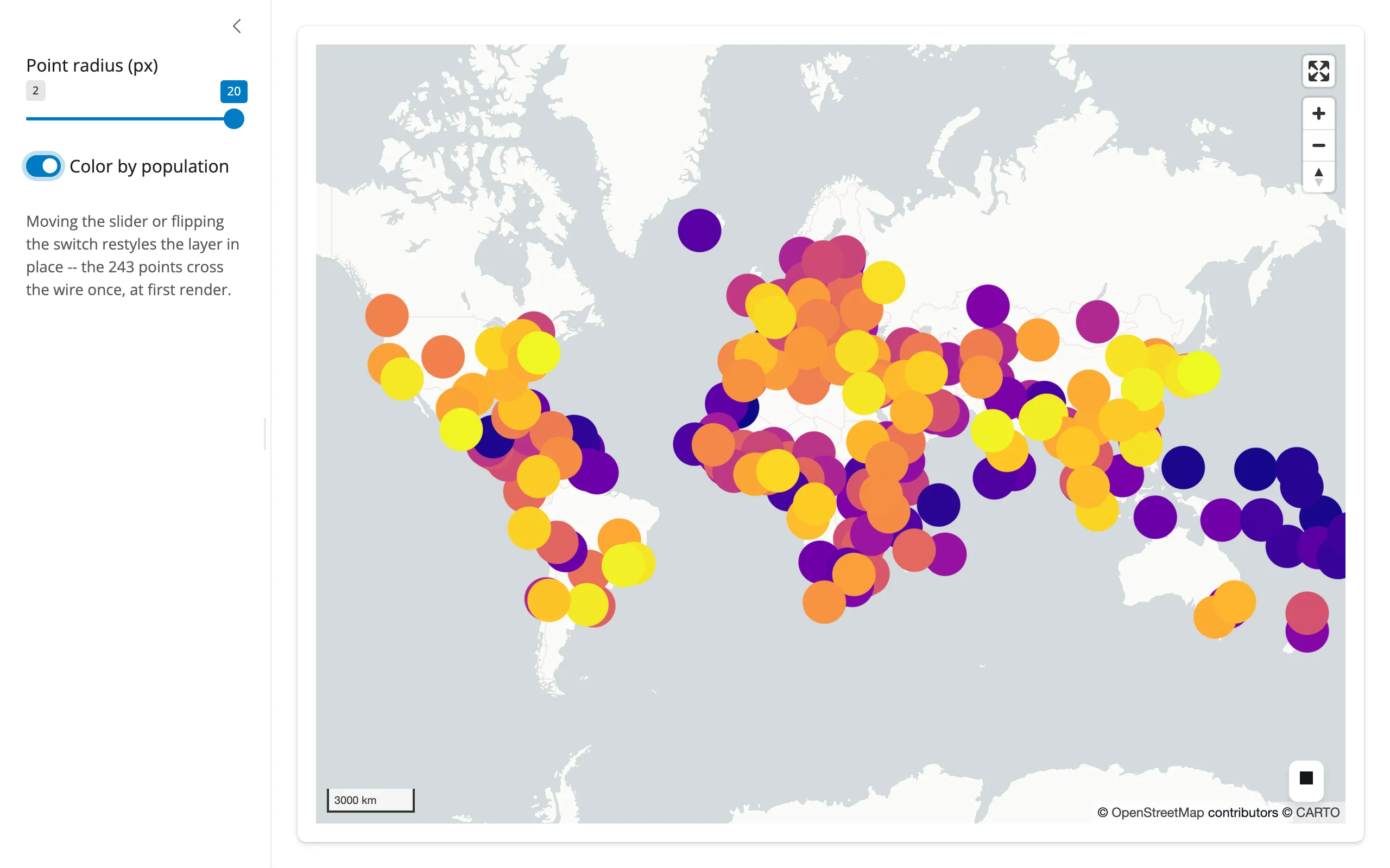
• map.widget.fly_to(...) animates the camera. Nothing about the data changes, so nothing is re-sent – selection state, styling, and the 243-point (or 243,000-point) buffer already in the browser are untouched.
• layer.trait = ... under reactive.isolate() restyles in place: only the changed trait (a color array, a radius) crosses the wire, not the geometry.

Both beat re-rendering, which rebuilds the Map from scratch, re-sends every point, and resets the camera to the new map’s own fitted view – losing whatever the user had panned or zoomed to.

Restyling in place

Read styling inputs under reactive.isolate() inside the render function (so the render only re-runs when the data changes), then push style updates from separate effects keyed to those inputs:

examples/09_restyle_in_place.py56 lines

import geopandas as gpd
import matplotlib.pyplot as plt
from lonboard import ScatterplotLayer
from lonboard.colormap import apply_continuous_cmap
from shiny import reactive
from shiny.express import input, ui
from shinywidgets import render_lonboard

ui.page_opts(fillable=True)

CITIES_URL = "https://raw.githubusercontent.com/nvkelso/natural-earth-vector/master/geojson/ne_110m_populated_places.geojson"

with ui.sidebar():
    ui.input_slider("radius", "Point radius (px)", 2, 20, 6)
    ui.input_switch("by_pop", "Color by population", False)
    ui.p(
        "Moving the slider or flipping the switch restyles the layer in "
        "place -- the 243 points cross the wire once, at first render.",
        class_="text-muted small",
    )

with ui.card(full_screen=True):

    @render_lonboard
    def map():
        # Read styling inputs under isolate(): this render function should
        # only re-run when the data changes, not on every slider tick
        with reactive.isolate():
            style = {"get_fill_color": fill_color(), "radius_min_pixels": input.radius()}
        return ScatterplotLayer.from_geopandas(cities(), **style)


@reactive.calc
def cities() -> gpd.GeoDataFrame:
    return gpd.read_file(CITIES_URL)


def fill_color():
    if not input.by_pop():
        return [255, 60, 120]
    pct = cities()["POP_MAX"].rank(pct=True).to_numpy()
    return apply_continuous_cmap(pct, plt.get_cmap("plasma"))


@reactive.effect
@reactive.event(input.radius, ignore_init=True)
def _update_radius():
    layer = map.widget.layers[0]
    layer.radius_min_pixels = input.radius()


@reactive.effect
@reactive.event(input.by_pop, ignore_init=True)
def _update_color():
    layer = map.widget.layers[0]
    layer.get_fill_color = fill_color()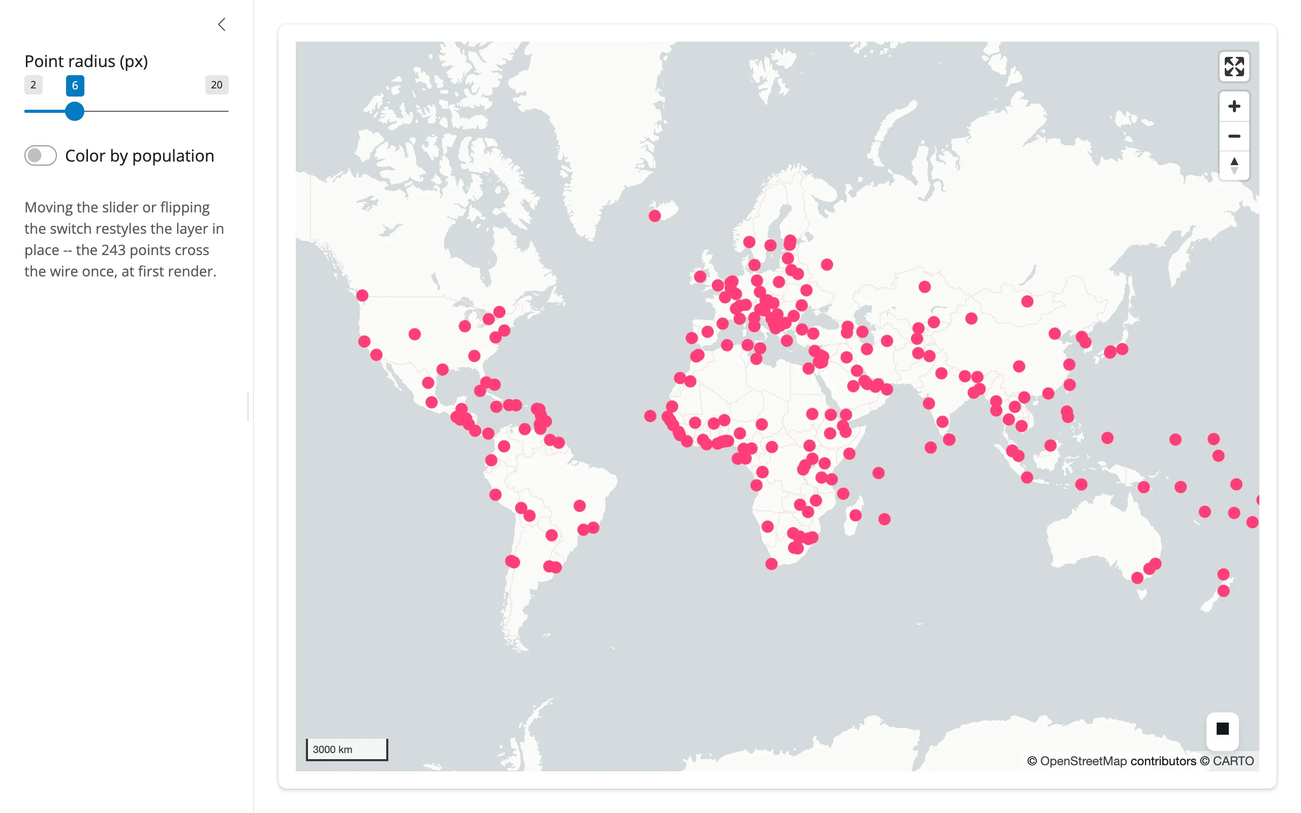

Flying the camera

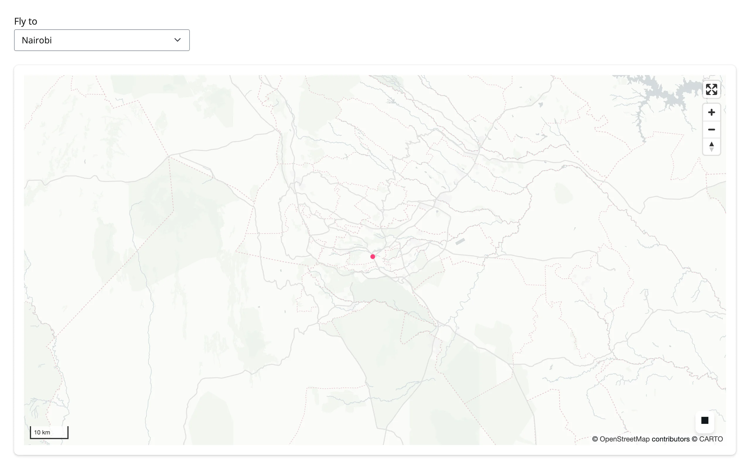
Map.fly_to(longitude=, latitude=, zoom=, duration=) animates the camera from Python – a search box, a “reset view” button, or (below) a table row selection:

examples/10_fly_to.py37 lines

import geopandas as gpd
from lonboard import ScatterplotLayer
from lonboard.view_state import MapViewState
from shiny import reactive
from shiny.express import input, ui
from shinywidgets import render_lonboard

ui.page_opts(fillable=True)

CITIES_URL = "https://raw.githubusercontent.com/nvkelso/natural-earth-vector/master/geojson/ne_110m_populated_places.geojson"
DESTINATIONS = {
    "Tokyo": (139.75, 35.68, 9),
    "Nairobi": (36.82, -1.29, 9),
    "Buenos Aires": (-58.38, -34.6, 9),
    "World": (10, 20, 1),
}

ui.input_select("city", "Fly to", list(DESTINATIONS))

with ui.card(full_screen=True):

    @render_lonboard
    def map():
        cities = gpd.read_file(CITIES_URL)
        layer = ScatterplotLayer.from_geopandas(
            cities, get_fill_color=[255, 60, 120], radius_min_pixels=4
        )
        return layer  # starts at the default world view


@reactive.effect
@reactive.event(input.city)
def _fly_to_city():
    lon, lat, zoom = DESTINATIONS[input.city()]
    # fly_to() animates the camera in the browser; it doesn't touch the
    # data, so nothing is re-sent and any selection/styling is preserved
    map.widget.fly_to(longitude=lon, latitude=lat, zoom=zoom, duration=1200)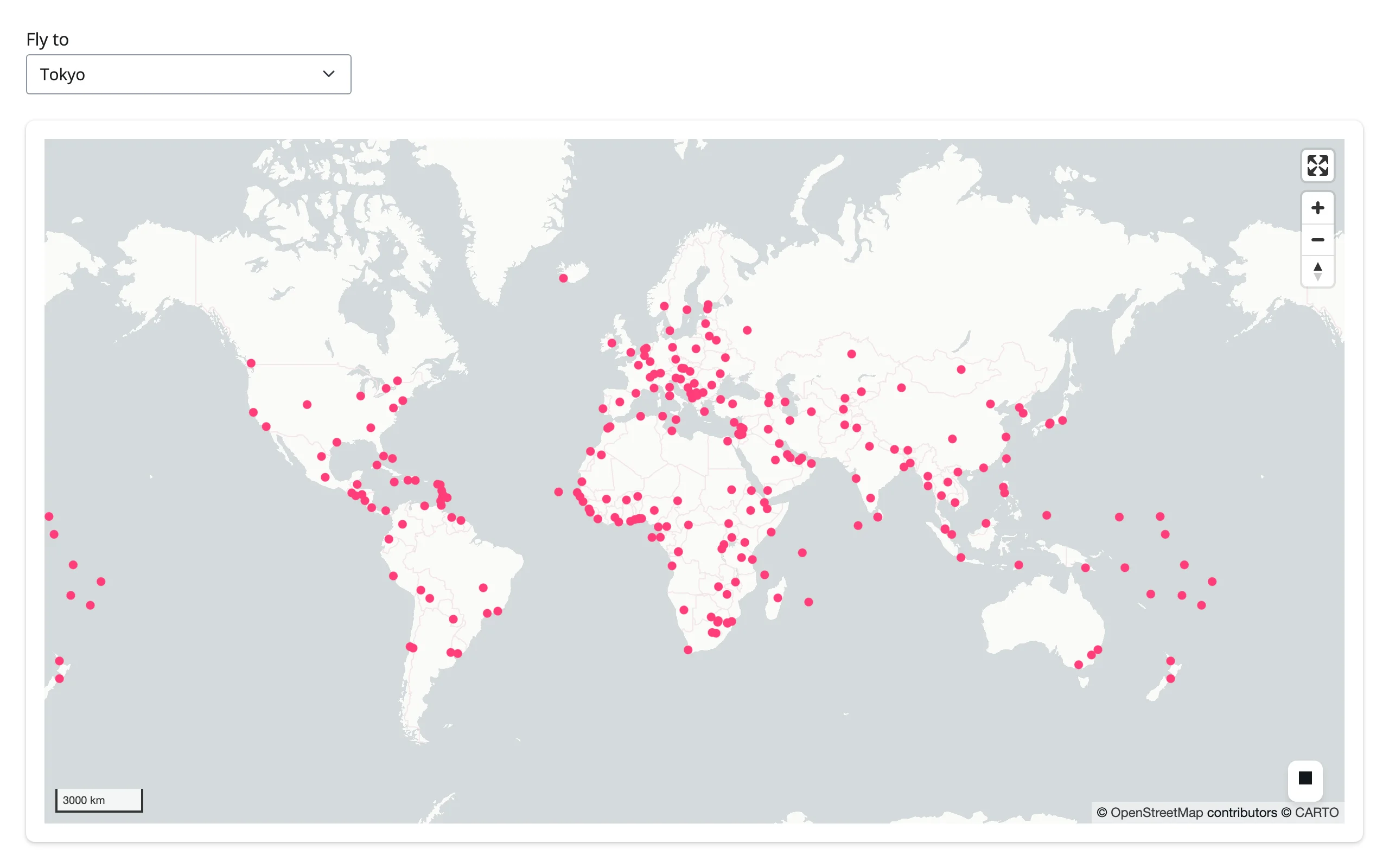

Coordinating multiple views

These four patterns are the most useful thing in this guide: the map drives a chart, a card, and a table, and a table drives the map back. Every one of them is driven entirely by the accessors above – no polling, no manual event wiring.

Viewport as a filter: map pans a chart

lonboard’s view_state has no bounds field (only center + zoom), so computing an exact lng/lat viewport box takes one more ingredient: the output’s on-screen pixel size, reported once (and on resize) by a tiny ResizeObserver script. Combine that with standard Web Mercator math and view_state() becomes an exact “what’s on screen” filter – here, driving a plotly bar chart of the largest cities currently in view.

examples/11_viewport_to_chart.py71 lines

import math

import geopandas as gpd
import plotly.express as px
from lonboard import ScatterplotLayer
from shapely.geometry import box
from shiny import req
from shiny.express import input, ui
from shinywidgets import render_lonboard, render_plotly

ui.page_opts(fillable=True)

CITIES_URL = "https://raw.githubusercontent.com/nvkelso/natural-earth-vector/master/geojson/ne_110m_populated_places.geojson"

# lonboard's view_state has no bounds field (only center + zoom), so compute
# the viewport's lng/lat box from Web Mercator math, using the output's
# on-screen pixel size (reported once and on every resize).
ui.head_content(
    ui.tags.script("""
    $(document).on("shiny:connected", function() {
      function send() {
        var el = document.querySelector("#map");
        if (el) Shiny.setInputValue("map_px", [el.clientWidth, el.clientHeight]);
      }
      new ResizeObserver(send).observe(document.body);
      setTimeout(send, 300);
    });
    """)
)

with ui.layout_columns(col_widths=[7, 5]):
    with ui.card(full_screen=True):

        @render_lonboard
        def map():
            cities = gpd.read_file(CITIES_URL)
            return ScatterplotLayer.from_geopandas(
                cities, get_fill_color=[255, 60, 120], radius_min_pixels=4
            )

    with ui.card():
        ui.card_header("Largest cities currently in view")

        @render_plotly
        def chart():
            vs = map.view_state()
            width, height = req(input.map_px())
            bounds = view_bounds(vs.longitude, vs.latitude, vs.zoom, width, height)
            cities = gpd.read_file(CITIES_URL)
            visible = cities[cities.geometry.within(box(*bounds))]
            top = visible.nlargest(12, "POP_MAX").sort_values("POP_MAX")
            fig = px.bar(top, x="POP_MAX", y="NAME", orientation="h")
            fig.update_layout(
                title=f"{len(visible)} cities in view", margin=dict(l=10, r=10, t=40, b=10)
            )
            return fig


def inv_merc(y: float) -> float:
    return math.degrees(2 * math.atan(math.exp(y)) - math.pi / 2)


def view_bounds(
    lon: float, lat: float, zoom: float, width: float, height: float
) -> tuple[float, float, float, float]:
    """(minx, miny, maxx, maxy) of a Web Mercator viewport (512px tiles)."""
    world_px = 512 * 2**zoom
    half_w = (width / 2) * 360 / world_px
    half_h = (height / 2) * (2 * math.pi) / world_px
    m = math.log(math.tan(math.pi / 4 + math.radians(lat) / 2))
    return (lon - half_w, inv_merc(m - half_h), lon + half_w, inv_merc(m + half_h))

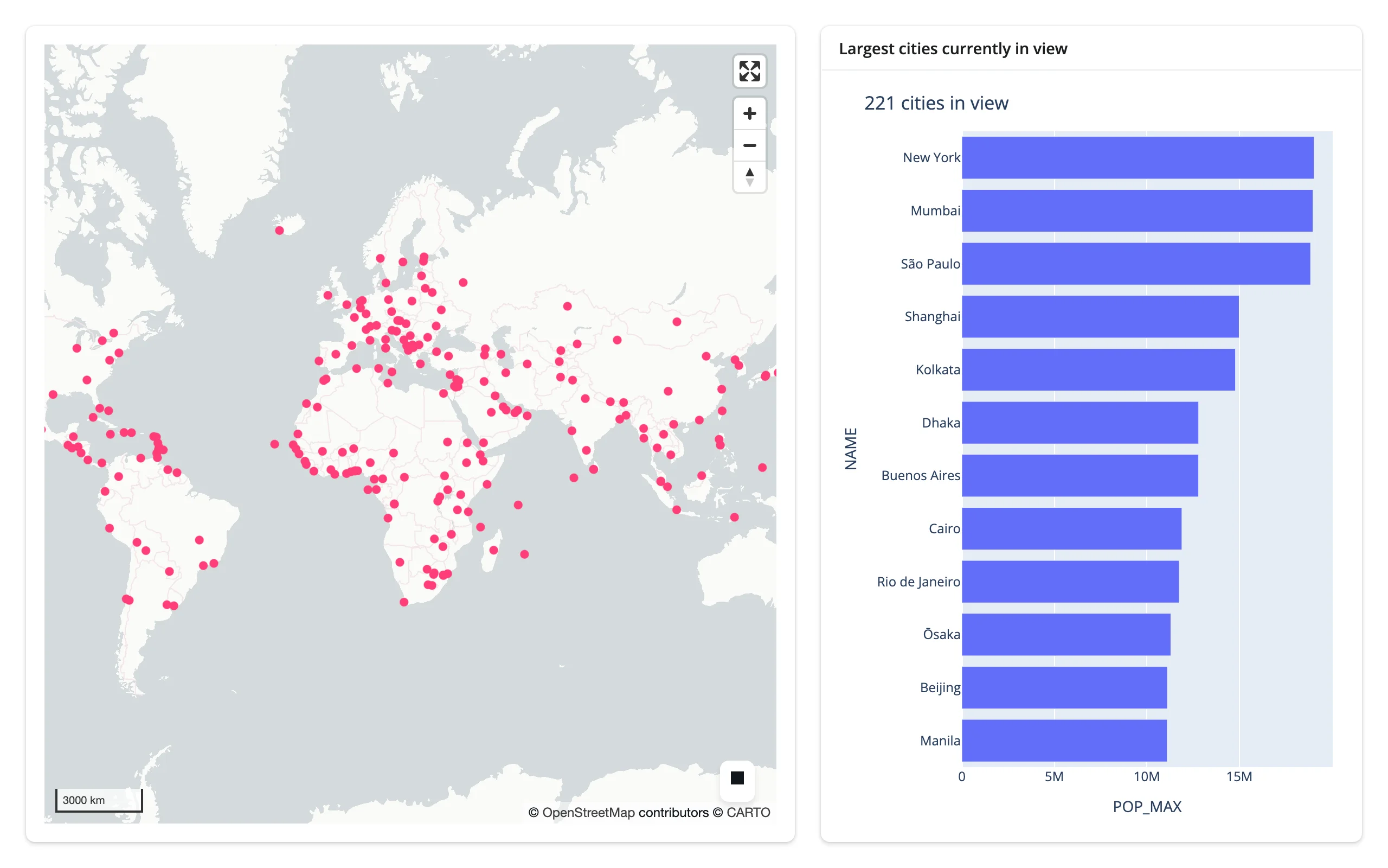
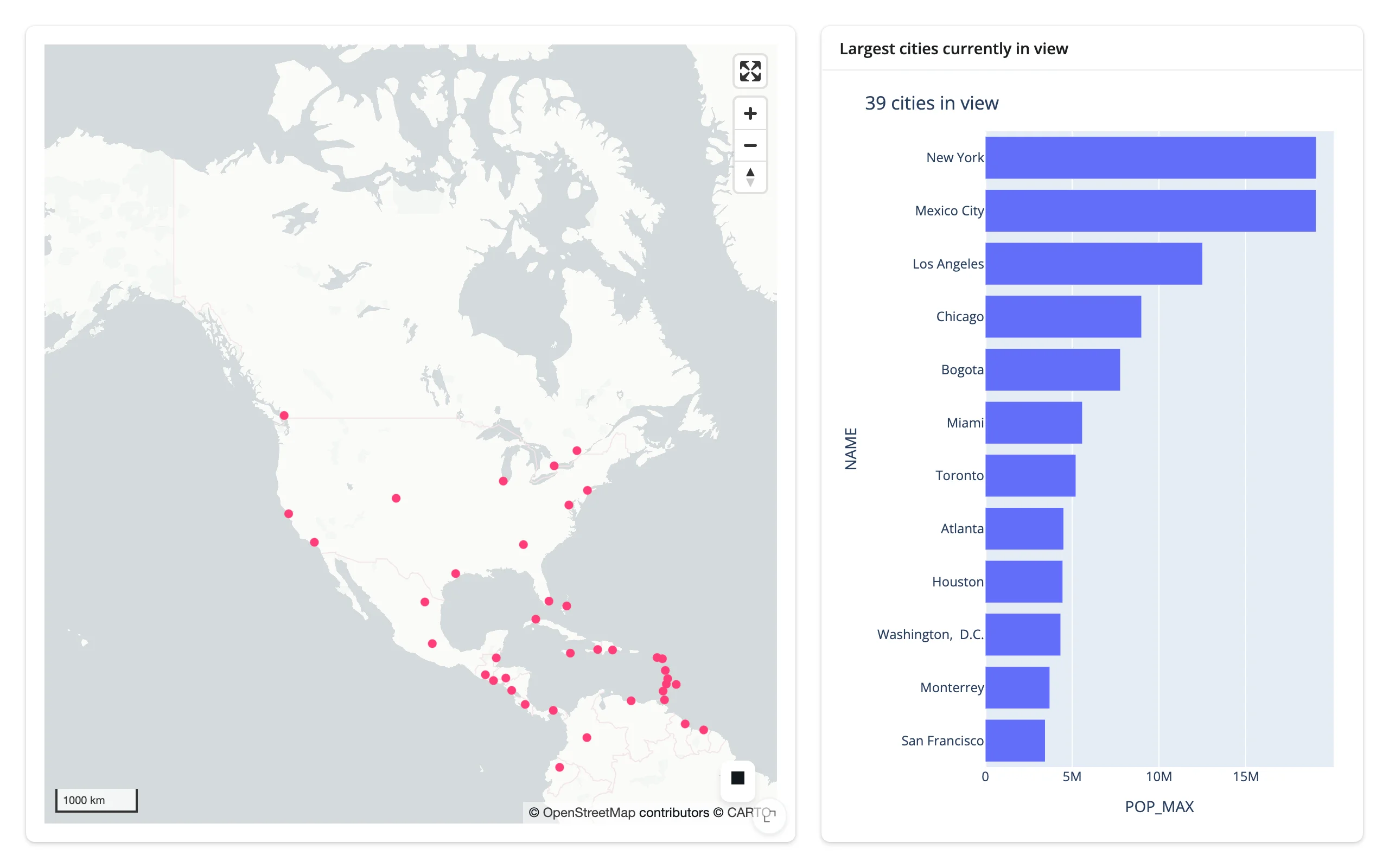
Pan and zoom, and the chart recomputes: 221 cities worldwide on load, down to 39 (and a different top-12) once the view is centered on North America.

pairs with: plotly

Click a city, see a detail card

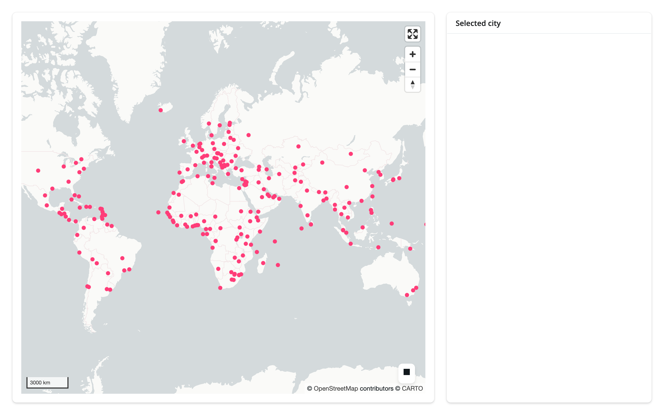
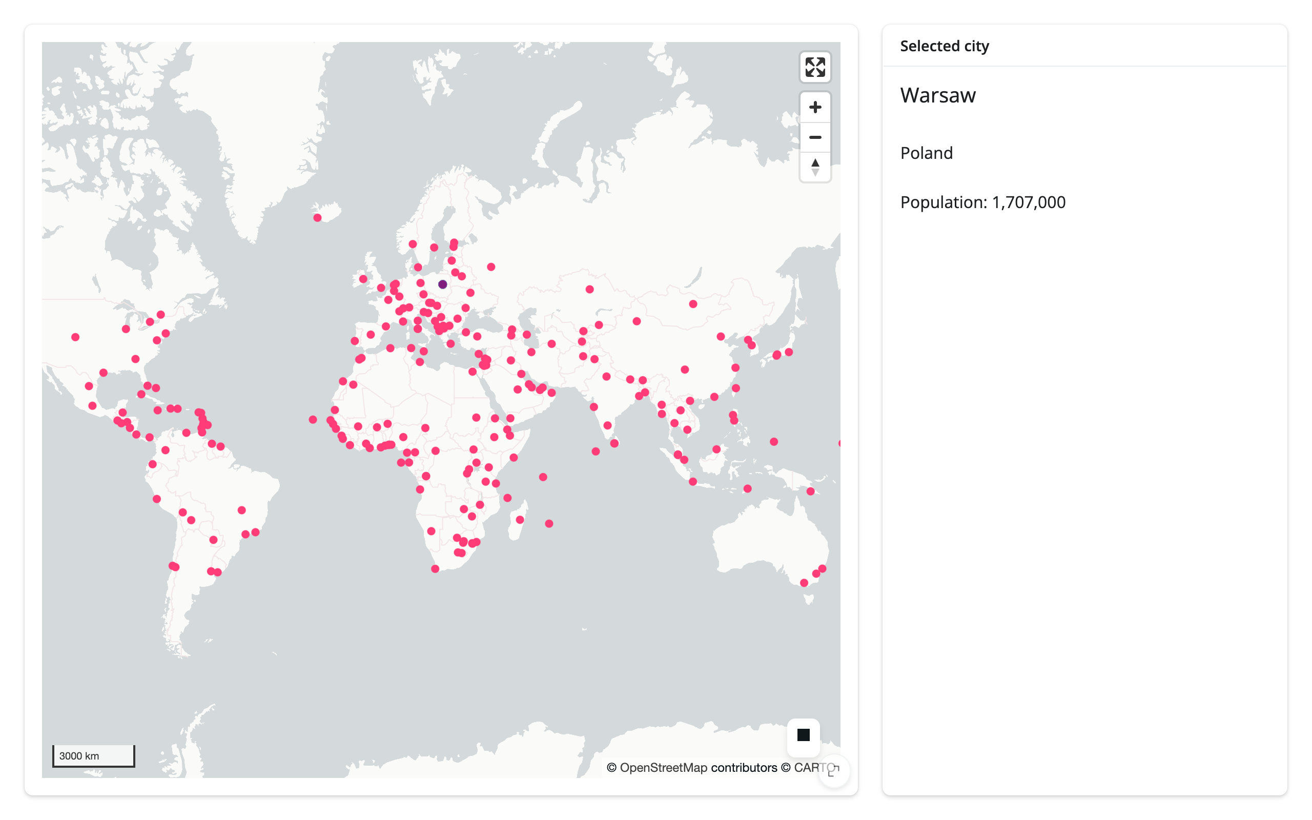
selected_rows() plus req() is the whole pattern: wait for the picked row, then show it. With no df argument the row comes from the layer’s own data, so the card doesn’t even re-read the file.

examples/12_click_to_detail_card.py44 lines

import geopandas as gpd
from lonboard import Map, ScatterplotLayer
from shiny import req
from shiny.express import render, ui
from shinywidgets import render_lonboard

ui.page_opts(fillable=True)

CITIES_URL = "https://raw.githubusercontent.com/nvkelso/natural-earth-vector/master/geojson/ne_110m_populated_places.geojson"


with ui.layout_columns(col_widths=[8, 4]):
    with ui.card(full_screen=True):

        @render_lonboard
        def map():
            cities = gpd.read_file(CITIES_URL)
            layer = ScatterplotLayer.from_geopandas(
                cities,
                get_fill_color=[255, 60, 120],
                radius_min_pixels=4,
                pickable=True,
                auto_highlight=True,
            )
            # The "Selected city" card already shows feature detail
            return Map(layer, show_side_panel=False)

    with ui.card():
        ui.card_header("Selected city")

        @render.ui
        def detail():
            # selected_rows() is the picked row itself, taken from the
            # layer's own data -- no second read of the file, no iloc. It's
            # an empty frame until the first pick; req() waits instead of
            # showing an empty card on load.
            rows = map.selected_rows()
            req(len(rows) > 0)
            row = rows.iloc[0]
            return ui.TagList(
                ui.h5(row["NAME"]),
                ui.p(row["ADM0NAME"]),
                ui.p(f"Population: {int(row['POP_MAX']):,}"),
            )

Box-select, see a filtered table

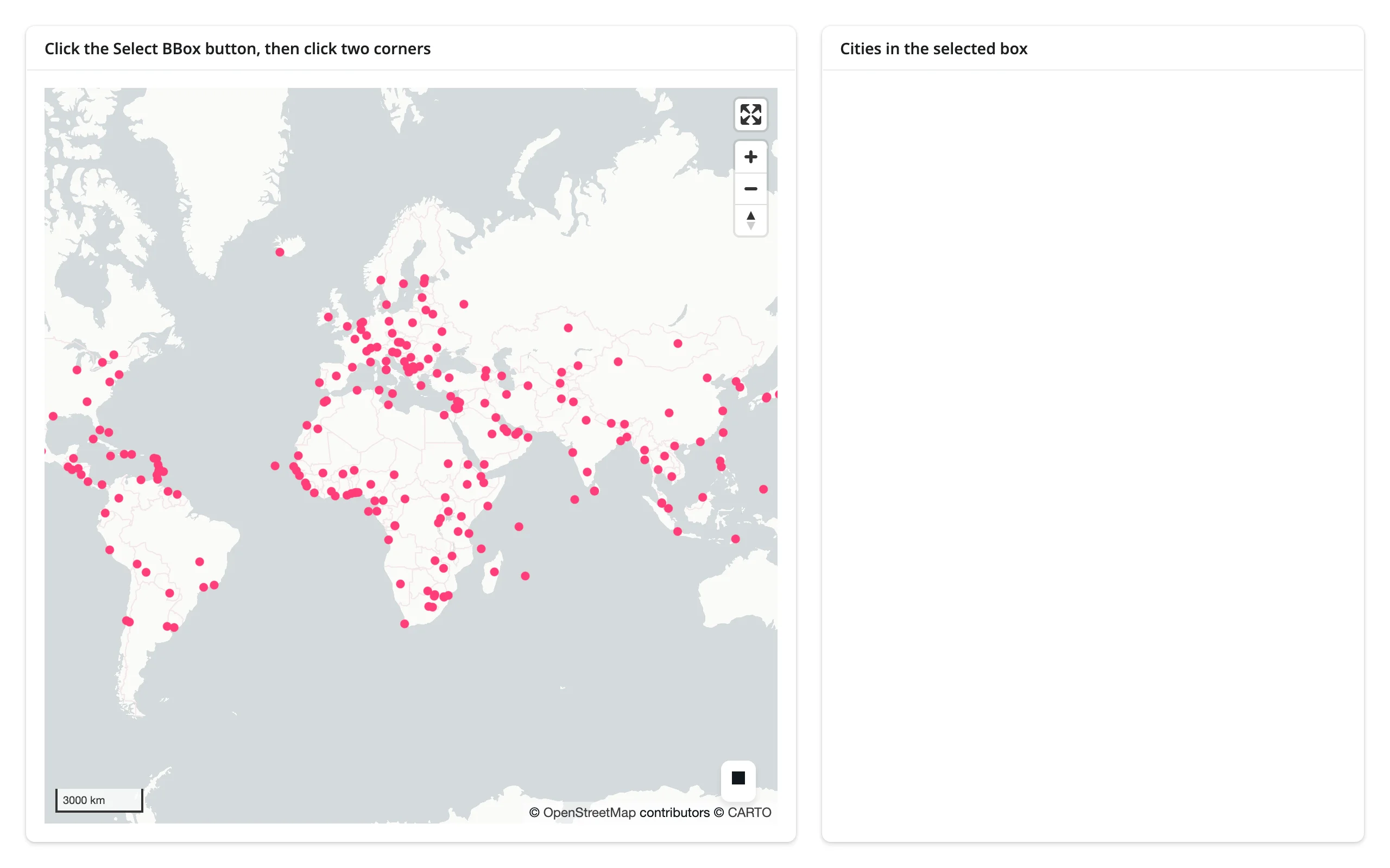
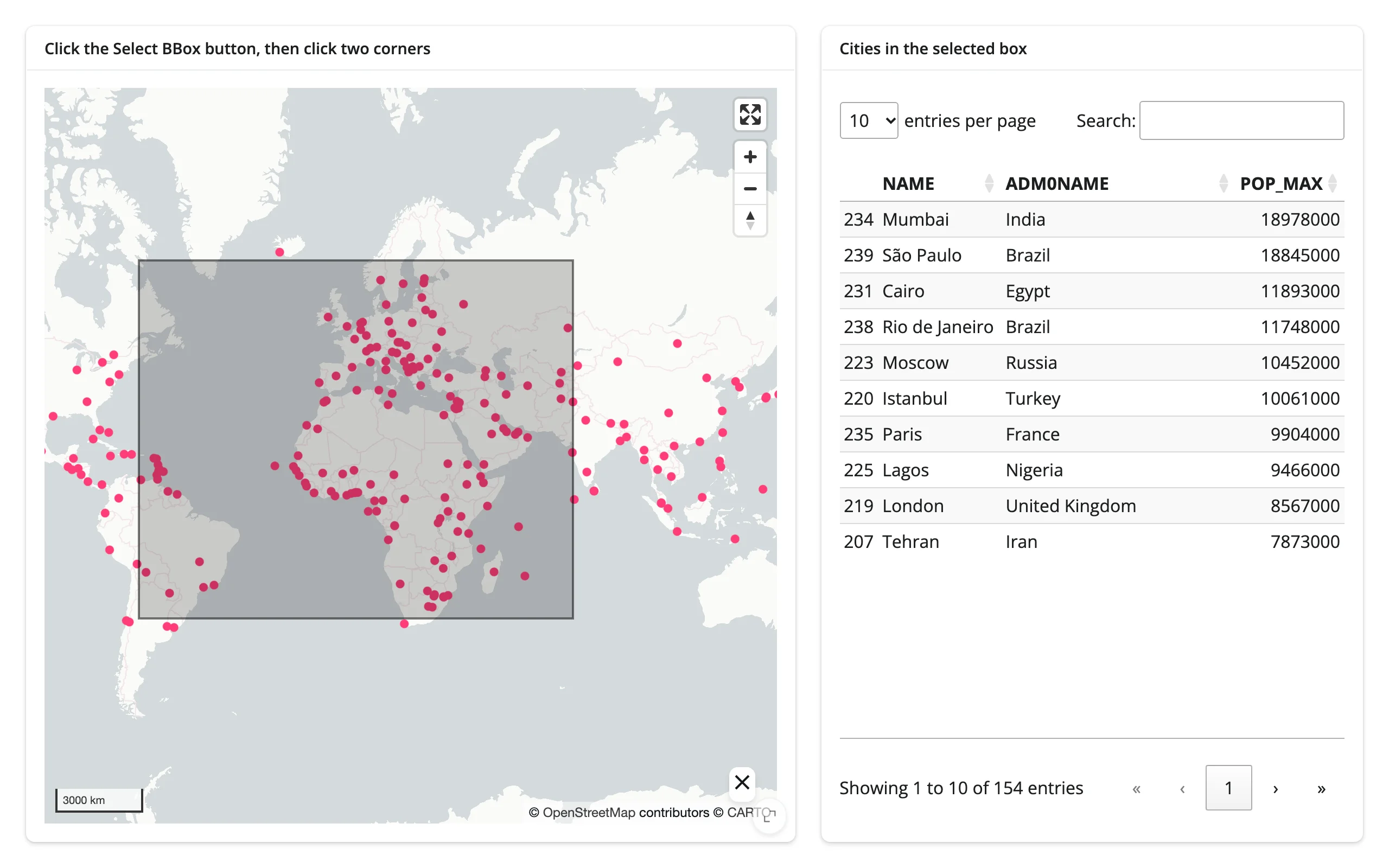
The same req() pattern, with selected_bounds() instead – and an itables output instead of a card.

examples/13_bbox_to_table.py34 lines

import geopandas as gpd
from lonboard import Map, ScatterplotLayer
from shapely.geometry import box
from shiny import req
from shiny.express import ui
from shinywidgets import render_itables, render_lonboard

ui.page_opts(fillable=True)

CITIES_URL = "https://raw.githubusercontent.com/nvkelso/natural-earth-vector/master/geojson/ne_110m_populated_places.geojson"

with ui.layout_columns(col_widths=[7, 5]):
    with ui.card(full_screen=True):
        ui.card_header("Click the Select BBox button, then click two corners")

        @render_lonboard
        def map():
            cities = gpd.read_file(CITIES_URL)
            layer = ScatterplotLayer.from_geopandas(
                cities, get_fill_color=[255, 60, 120], radius_min_pixels=4
            )
            return Map(layer, show_side_panel=False)

    with ui.card():
        ui.card_header("Cities in the selected box")

        @render_itables
        def table():
            bounds = req(map.selected_bounds())
            cities = gpd.read_file(CITIES_URL)
            selected = cities[cities.geometry.within(box(*bounds))]
            return selected[["NAME", "ADM0NAME", "POP_MAX"]].sort_values(
                "POP_MAX", ascending=False
            )

pairs with: itables

The other direction: a table row flies the map

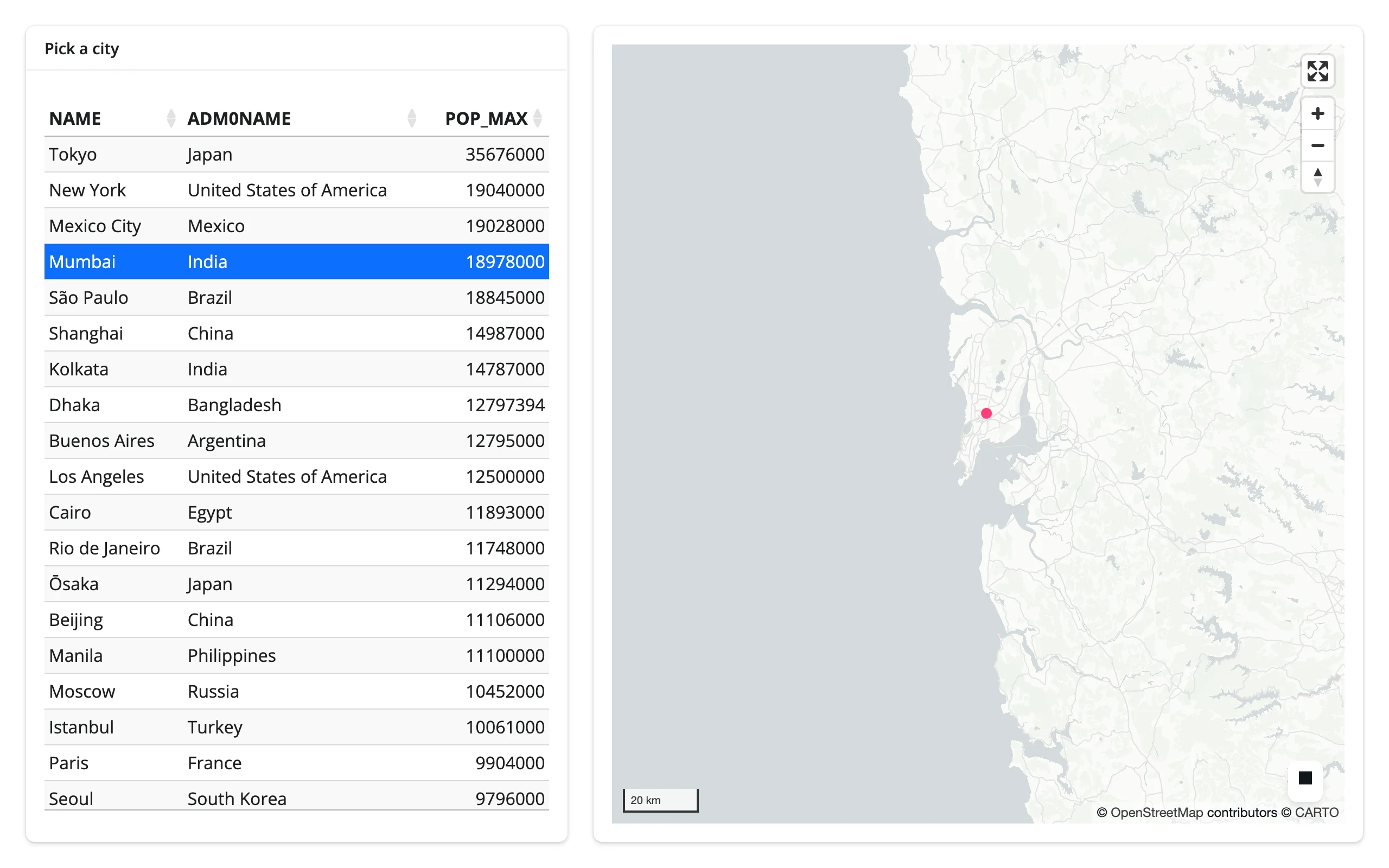
Interaction isn’t one-way. An itables row selection (table.selected_rows()) drives map.widget.fly_to(...) – the map is the one being updated here, in place, with its existing styling and the other table’s selection state untouched.

examples/14_table_to_fly_to.py42 lines

import geopandas as gpd
from itables.widget import ITable
from lonboard import ScatterplotLayer
from shiny import reactive, req
from shiny.express import ui
from shinywidgets import render_itables, render_lonboard

ui.page_opts(fillable=True)

CITIES_URL = "https://raw.githubusercontent.com/nvkelso/natural-earth-vector/master/geojson/ne_110m_populated_places.geojson"


@reactive.calc
def cities() -> gpd.GeoDataFrame:
    return gpd.read_file(CITIES_URL).nlargest(20, "POP_MAX").reset_index(drop=True)


with ui.layout_columns(col_widths=[5, 7]):
    with ui.card():
        ui.card_header("Pick a city")

        @render_itables
        def table():
            df = cities()[["NAME", "ADM0NAME", "POP_MAX"]]
            return ITable(df, select=True, lengthMenu=[20])

    with ui.card(full_screen=True):

        @render_lonboard
        def map():
            return ScatterplotLayer.from_geopandas(
                cities(), get_fill_color=[255, 60, 120], radius_min_pixels=5
            )


@reactive.effect
def _fly_to_selected():
    rows = req(table.selected_rows())
    row = cities().iloc[rows[0]]
    # table drives the map: selecting a row flies the camera there, without
    # re-sending the 20 points or losing any in-place styling
    map.widget.fly_to(longitude=row.LONGITUDE, latitude=row.LATITUDE, zoom=8, duration=1200)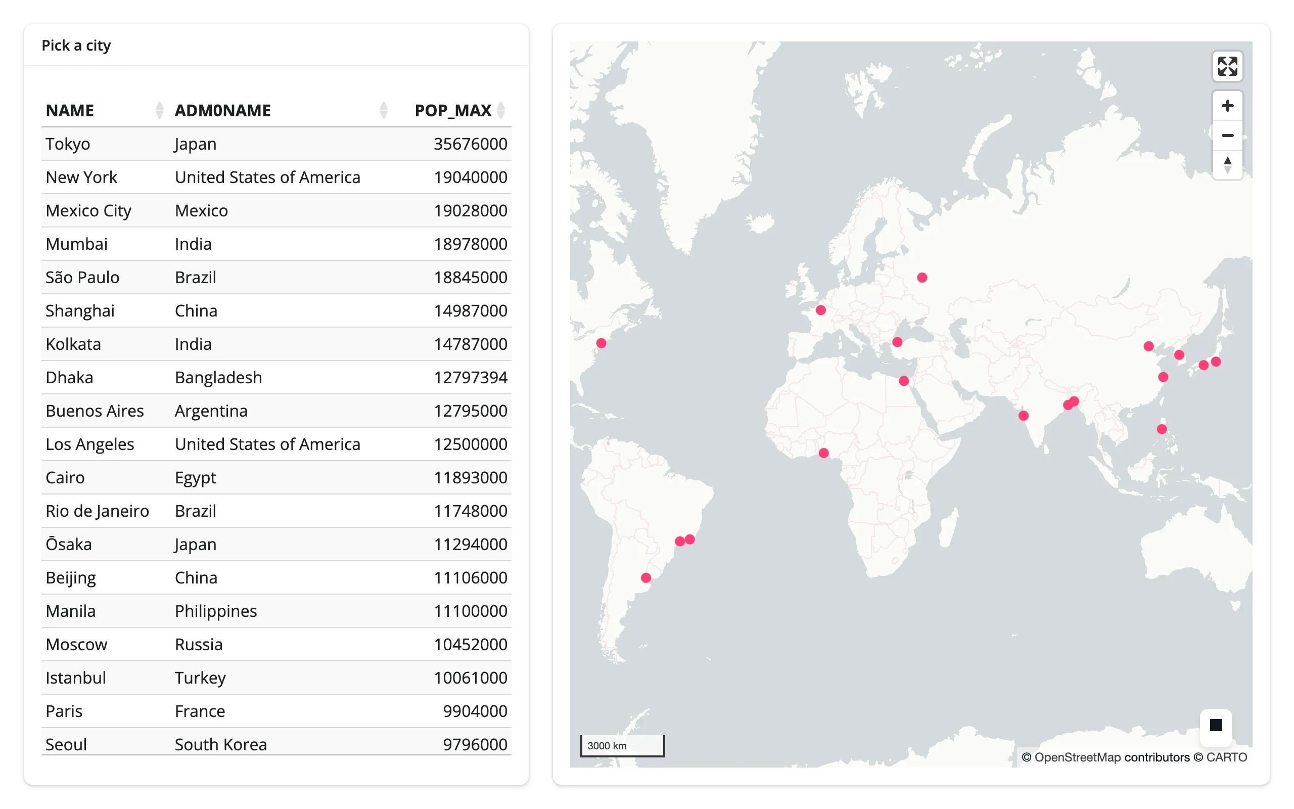

pairs with: itables

Large data

lonboard’s large-data mode is the renderer itself: GeoArrow-columnar data crosses the wire once and deck.gl draws it with WebGL, so pan, zoom, and restyle stay smooth regardless of point count – the GPU-in-browser approach. The Large data & performance article measured lonboard’s own initial payload and render time at 10K/100K/1M points: 25.2 MB and 3.1 s at 1M, the fastest of the three scatter renderers compared there (plotly 8.8 s, jscatter 3.7 s). lonboard doesn’t publish a hard ceiling beyond that; a few million points is where client-side GeoArrow decode and bundle cost are worth profiling on your own data rather than assuming it will stay smooth. See the three approaches for how this compares to summarizing on the server or sending only what’s visible.

Layout and sizing

lonboard has the best-in-class fill behavior in the shinywidgets roster: in a filling layout (the default), the map tracks its container’s size, including through window resizes and full_screen card enter/exit. The flip side is a trap worth knowing about:

• Percentage heights silently produce a blank map. Map(height="50%") renders a 0-height canvas – lonboard’s CSS gives the root element min-height: 100%, which is meaningless once the container itself isn’t a definite height. Use a pixel height (Map(height=400)), or leave height unset and let the output fill its container.
• An explicit pixel height that’s taller than its fillable row can overflow by the difference; the card clips or scrolls it. Cosmetic, and easy to avoid by not combining a tall fixed height with a short fillable row.
• With no definite height to fill and no explicit height, the map keeps lonboard’s own default (500 px) rather than collapsing.

Gotchas and limitations

Verified on current main (lonboard 0.17.0):

• GlobeView breaks view_state(). The browser’s view-state sync message always includes pitch/bearing (the same payload shape used for the regular Mercator view), but GlobeViewState has no pitch or bearing fields. The very first sync after a GlobeView map renders raises TypeError: GlobeViewState.__init__() got an unexpected keyword argument 'pitch' inside ipywidgets’ message handler – caught and logged, not fatal, but view_state() silently stops updating for globe maps from then on. This is an upstream lonboard bug, not something shinywidgets can paper over.
• Percentage heights silently collapse the map – see Layout and sizing.
• selected() can’t tell you which layer fired. With several pickable layers, read each layer’s own selected_index trait via reactive_read() instead (see Beyond the accessors). For the same reason, selected_rows()’s df default raises on such a map – pass df= for the layer you mean.
• Select BBox is click-click, not drag. Click the button, click one corner, click the opposite corner. Setting selected_bounds from Python doesn’t draw the overlay rectangle.
• view_state() can lag during an active zoom transition. The browser reports a new value on every frame of a wheel-zoom or double-click-zoom animation, and each one re-arms the 250 ms debounce, so view_state() doesn’t settle until the animation stops producing frames – longer for a multi-frame zoom transition than for a simple drag-pan.
• GlobeView is a private import (lonboard._map.GlobeView) – there’s no public top-level export for it yet.
• An older review of this integration reported that changing basemap after a fly-to desynced view_state from the visible map. That does not reproduce on current main: toggling basemap leaves the pre-existing pan/zoom in place and view_state() stays accurate. It appears to have been fixed upstream since that review; dropped from this list.

Gallery candidates

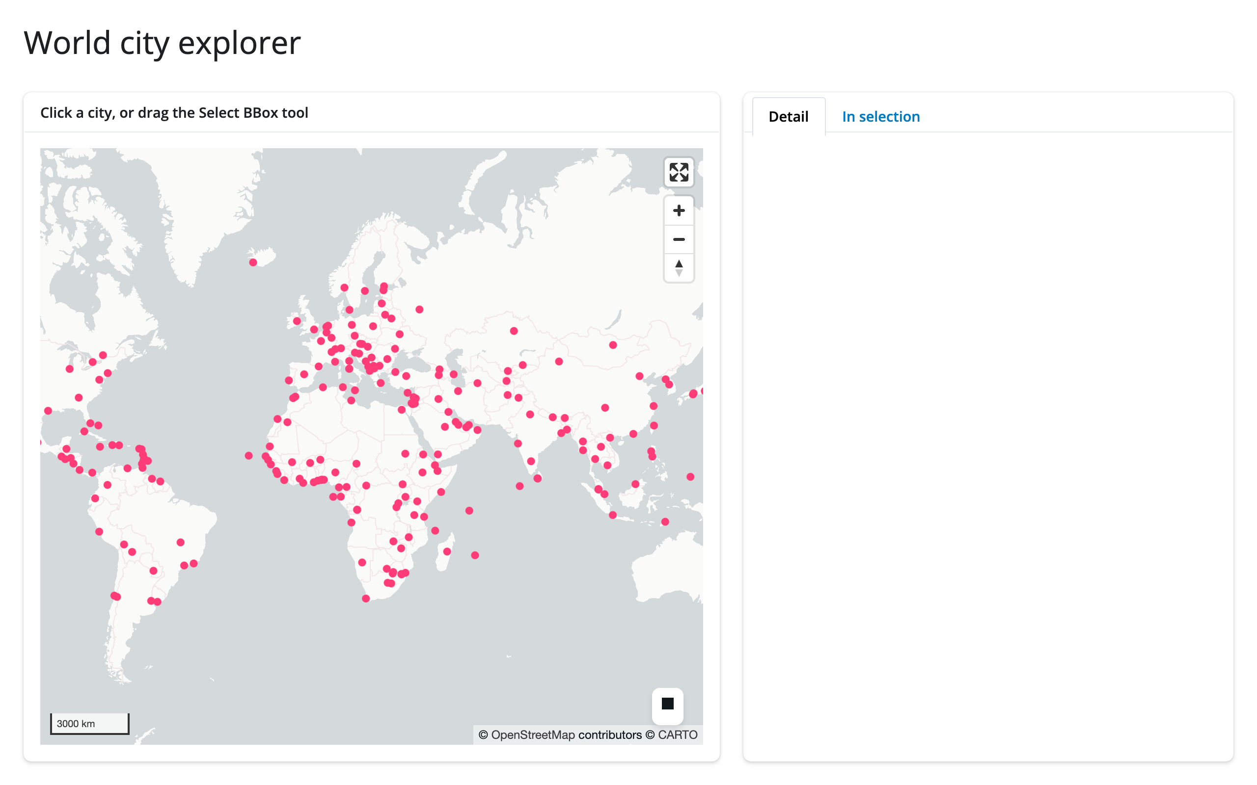
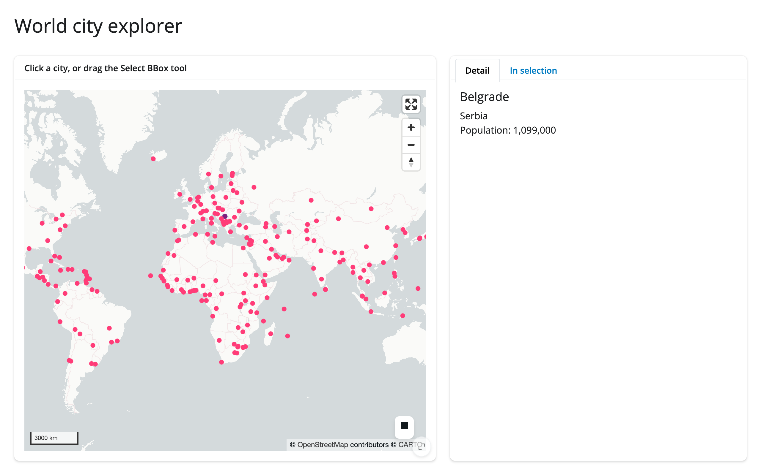
template_city_explorer.py (template) – a clean, ~65-line starting point: click a city for a detail card, or box-select for a filtered table, in tabs beside the map.

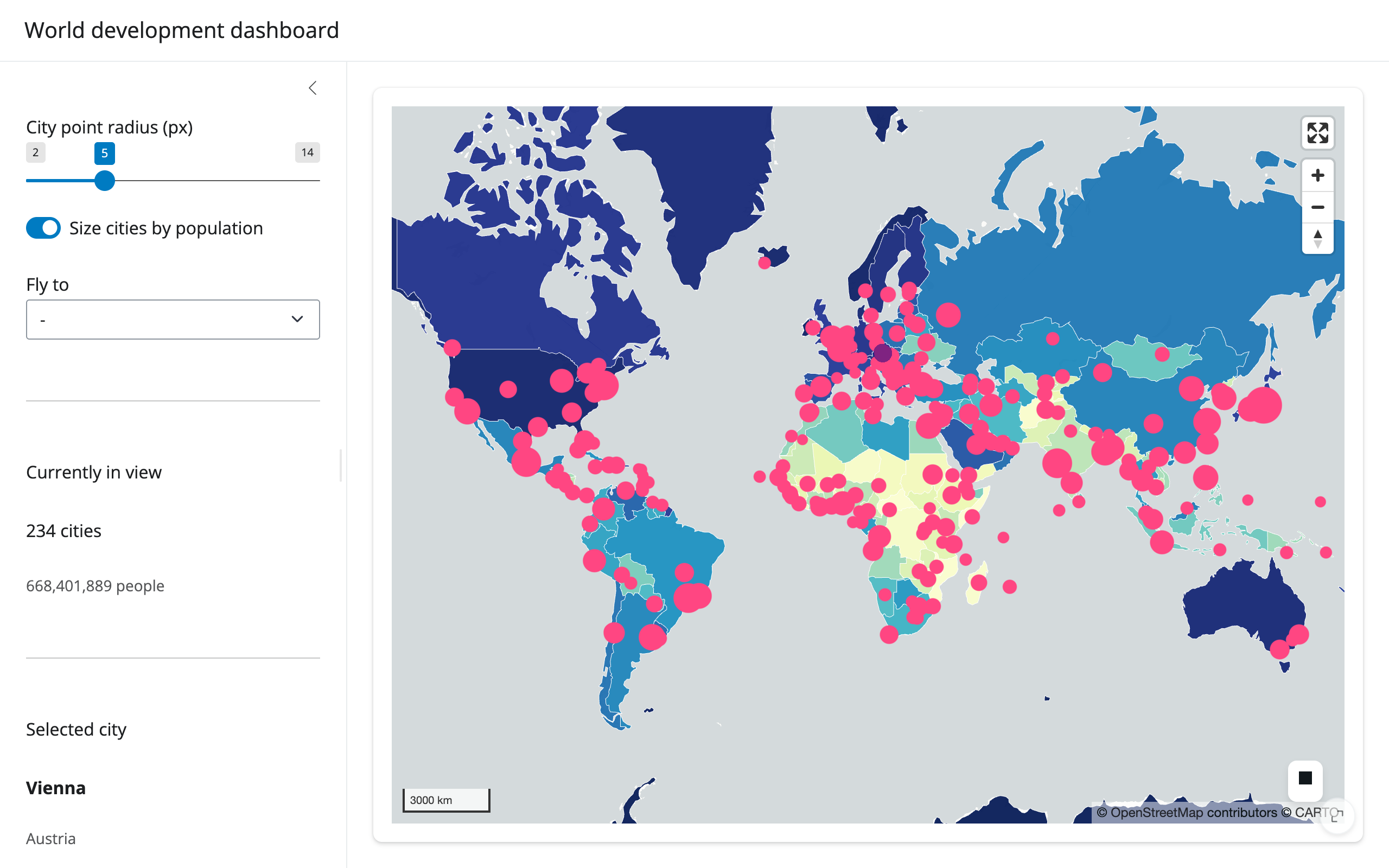
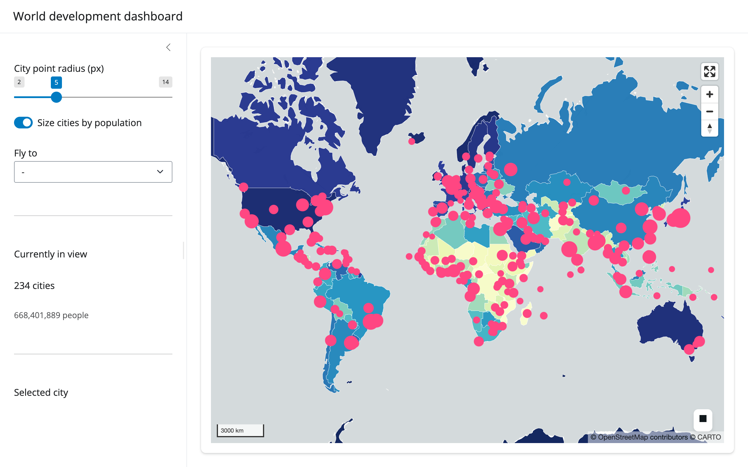
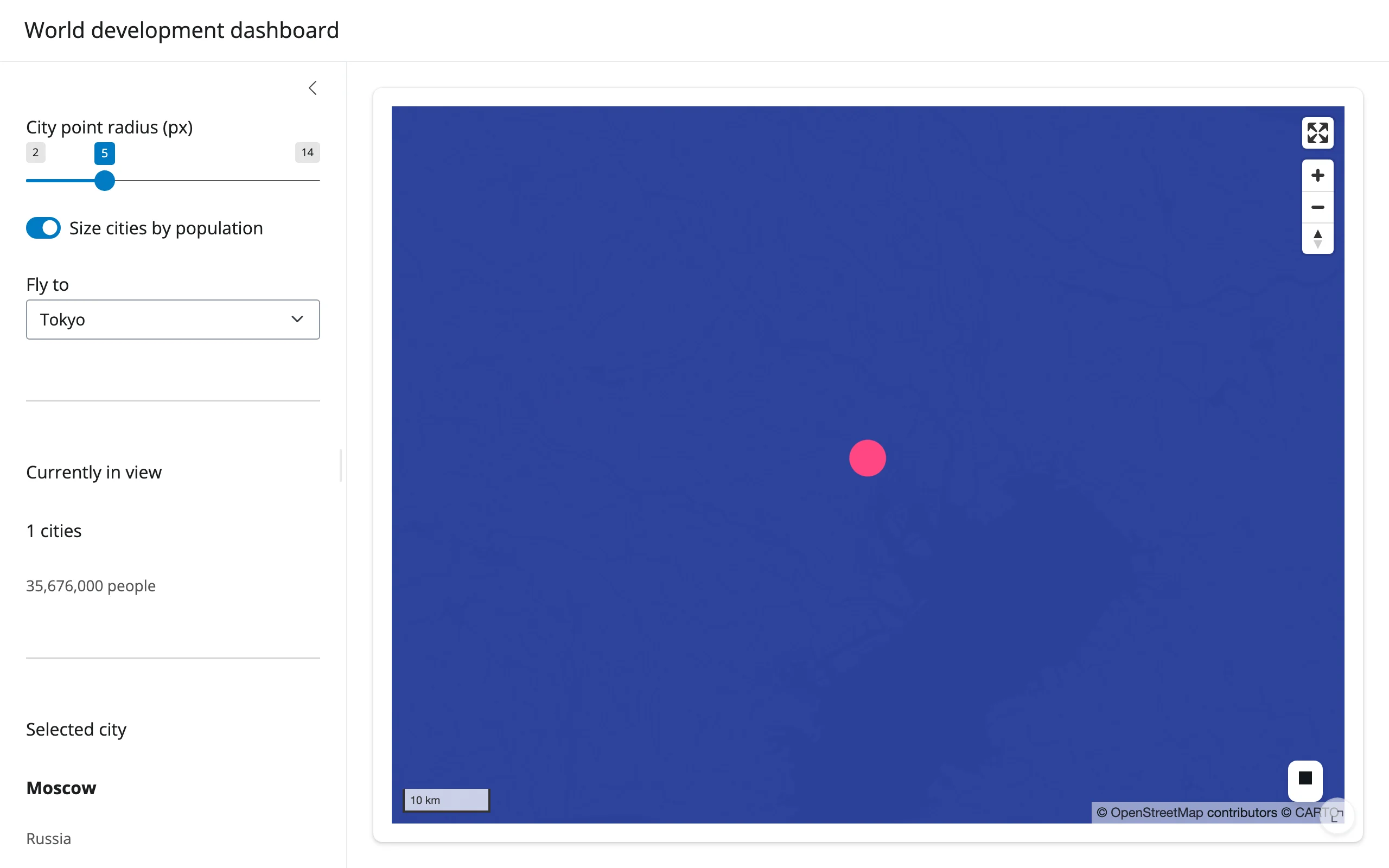
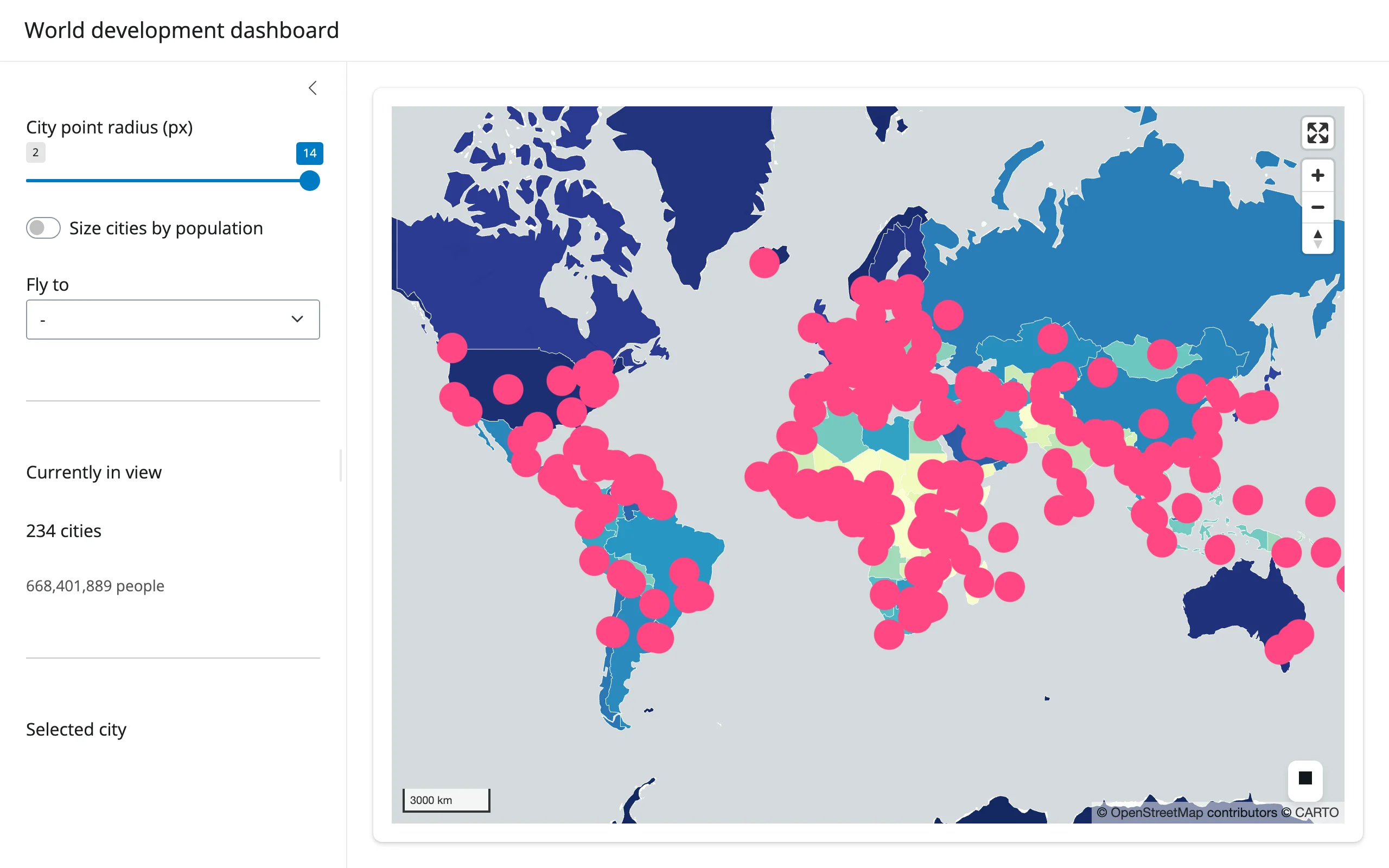
showcase_world_dashboard.py (showcase) – a GDP-per- capita choropleth (PolygonLayer + apply_continuous_cmap) with a population-scaled city layer on top. The sidebar’s “currently in view” stat comes from view_state() plus the Web Mercator viewport-bounds technique above; the detail card comes from selected_rows(cities()) (two pickable layers, so the frame is passed explicitly); the radius slider and population-size toggle restyle in place; and a “fly to” dropdown animates the camera to a handful of cities without touching the 420 rendered features.

Learn more

• lonboard documentation – full layer API reference, colormap gallery, and examples
• GeoArrow – the Arrow-native geometry format lonboard is built on
• deck.gl – the WebGL rendering engine underneath
• Related guides in this roster: ipyleaflet, leafmap, maplibre, keplergl, plotly, itables