drawdata
drawdata, by Vincent Warmerdam (koaning), is a tiny anywidget library with one job: let you draw a dataset by hand instead of loading one. ScatterWidget gives you a canvas where you drag a brush to lay down up to four classes of labeled 2D points; BarWidget gives you a histogram whose bars you drag up and down to sculpt a distribution. Both widgets were built for teaching – showing what a classifier’s decision boundary looks like, how an outlier drags a regression line, why k-means needs separated blobs to work – by letting the data itself be the thing you control.
@render_drawdata is a thin wrapper: it renders either widget with no coercion and no fixed accessors, and fixes one real layout bug (see below). The whole point of this guide is what you build around it – a second output that re-reads the drawing and reacts, from a point counter up to a live scikit-learn model. drawdata has no reactive accessor methods, so every example below reads the widget with canvas.read("data") – the generic way to reach a synced trait on any renderer output, documented in the render-widget guide.
Reach for drawdata when you want an interactive input that is a dataset – a teaching app, a quick “does this algorithm behave the way I expect” sandbox, or a way to generate a toy dataset without typing out coordinates. For drawing on top of an image or building a free-form annotation tool, see ipycanvas instead; drawdata’s canvas only ever produces points or bar heights, not arbitrary paths.
Installation
pip install 'shinywidgets[drawdata]'This installs drawdata (tested against 0.5.2). No other setup is required.
Quick start
from __future__ import annotations

from drawdata import ScatterWidget
from shiny.express import render, ui
from shinywidgets import render_drawdata

ui.page_opts(fillable=True)

with ui.card(full_screen=True):
    ui.card_header("Draw a dataset (pick a class, then drag)")

    @render_drawdata
    def canvas():
        return ScatterWidget(width=800, height=400, n_classes=2)


@render.code
def summary():
    # .read("data") re-runs this whenever a new drawing batch syncs; a
    # plain `canvas.widget.data` read would only ever see the first value.
    df = canvas.read("data")
    return f"{len(df)} points drawn"
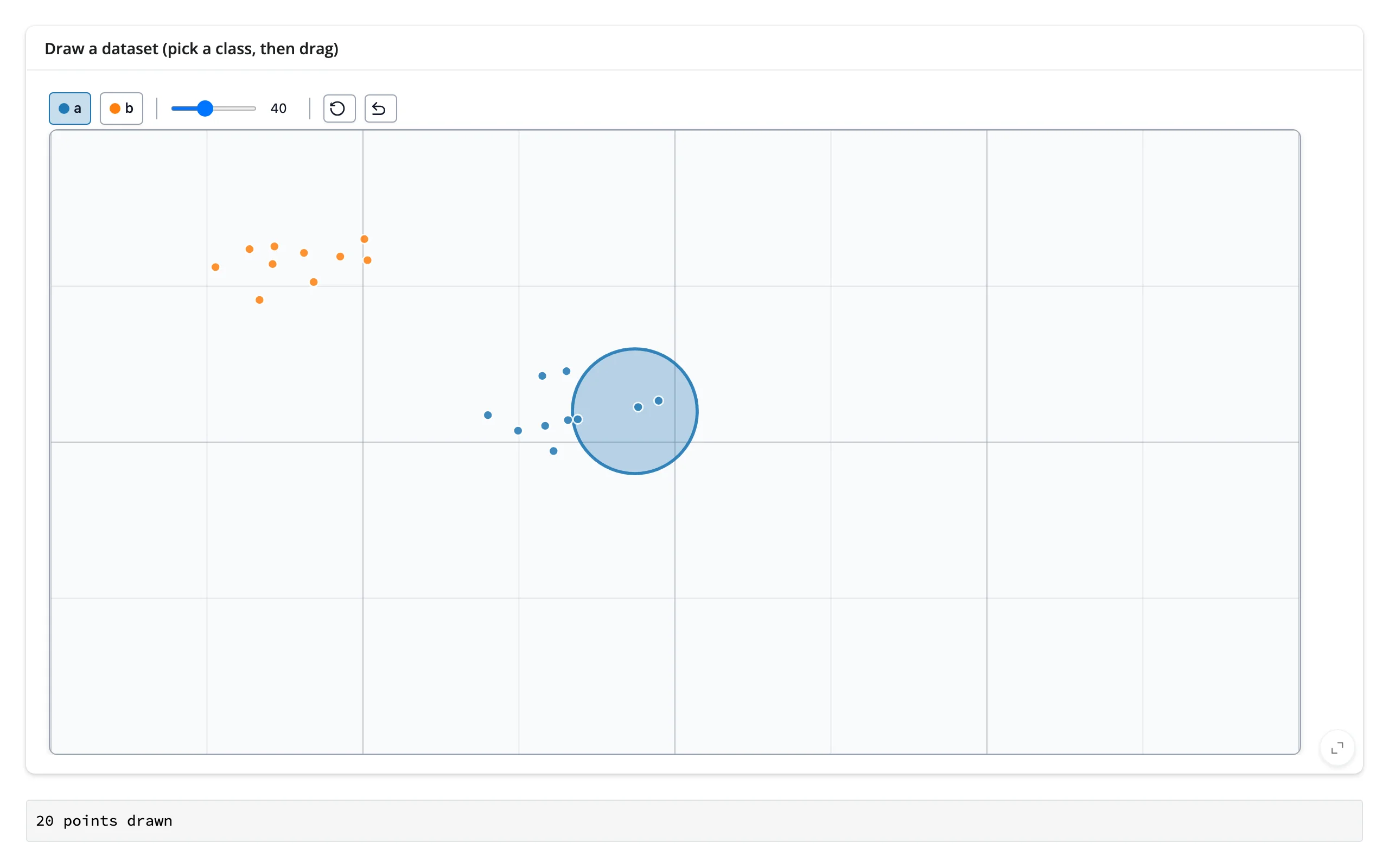
Pick a class (a or b), drag the brush across the canvas, and the point count below updates:
What you can build
A live DataFrame of everything drawn
Every stroke becomes rows in a plain Python list of dicts – {x, y, color, label, batch} – so a table of the drawing is a one-liner away. n_classes (1-4) is fixed at construction; change it by returning a new ScatterWidget.
        @render.data_frame
        def table():
            # canvas.widget.data_as_pandas is the same frame, but it's a plain
            # (non-reactive) property read -- it would compute once and never
            # update. Build the frame from .read("data") instead.
            data = canvas.read("data")
            return render.DataGrid(pd.DataFrame(data), height="100%")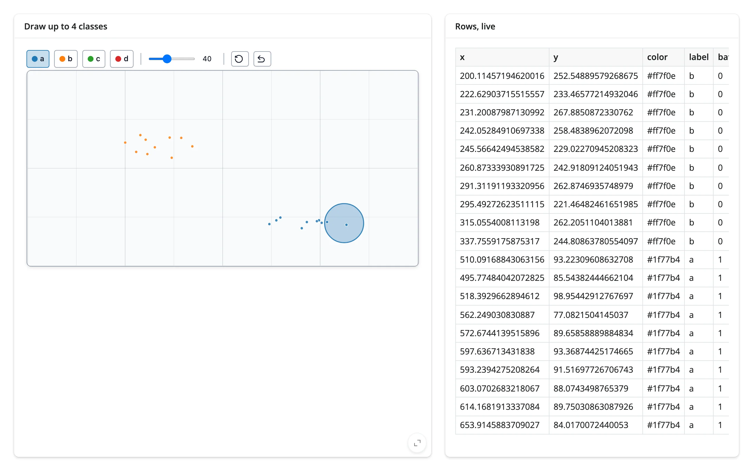
Sculpt a distribution by hand
BarWidget is the other half of the library: drag bars up and down to build a histogram shape instead of placing points. Pass a single-element collection_names to get one plain distribution (the default, ["collection1", "collection2"], gives you two switchable ones – see “Comparing two sculpted distributions” below).
        @render_drawdata
        def hist():
            # A single collection name hides the collection-switcher and
            # Clear buttons that show up with the default two names.
            return BarWidget(collection_names=["height_cm"], y_max=2.0, n_bins=20)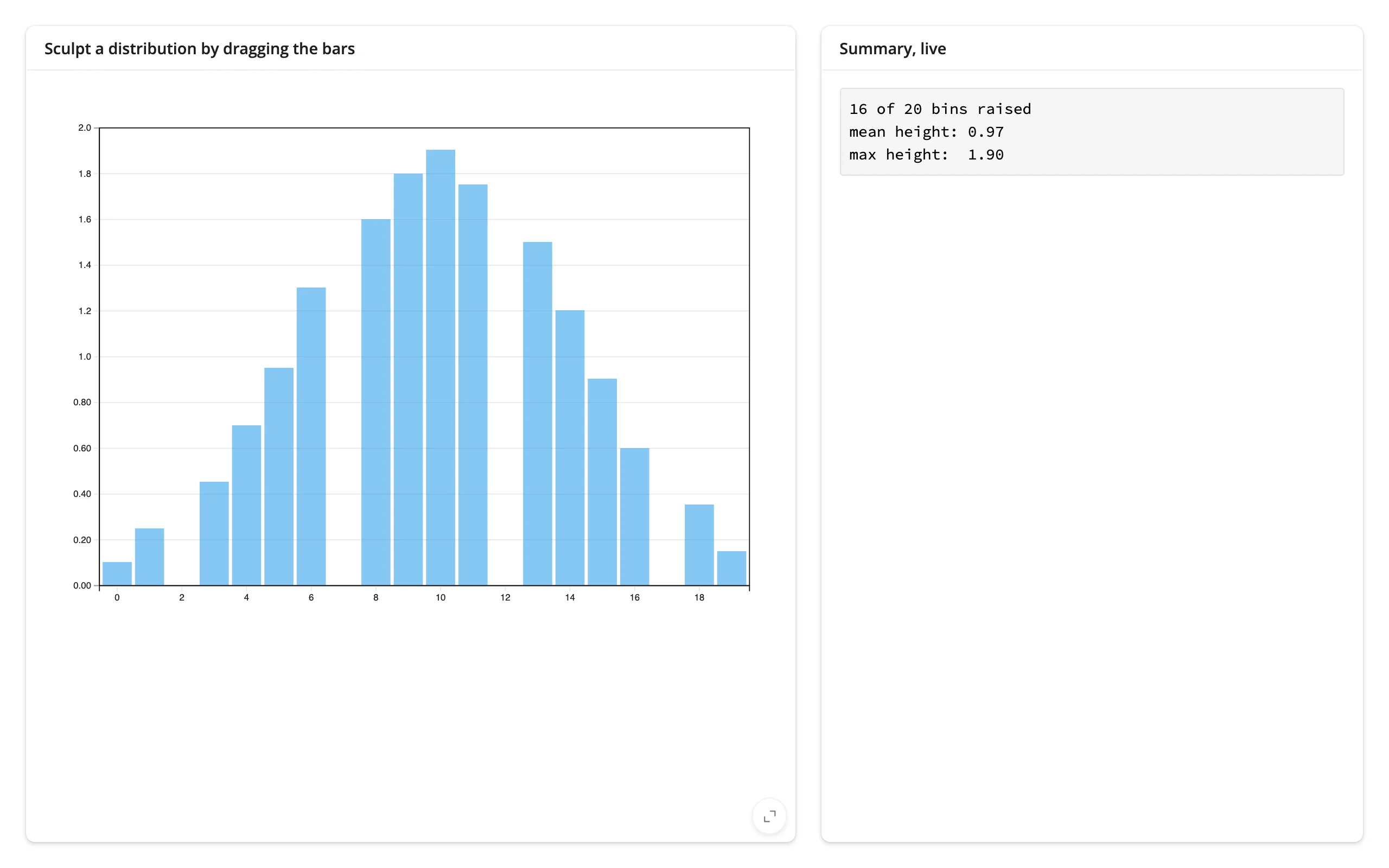
A live classifier decision boundary
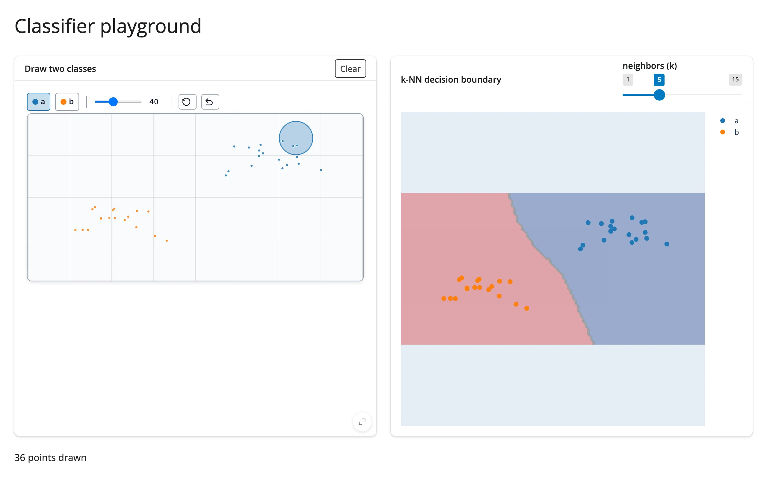
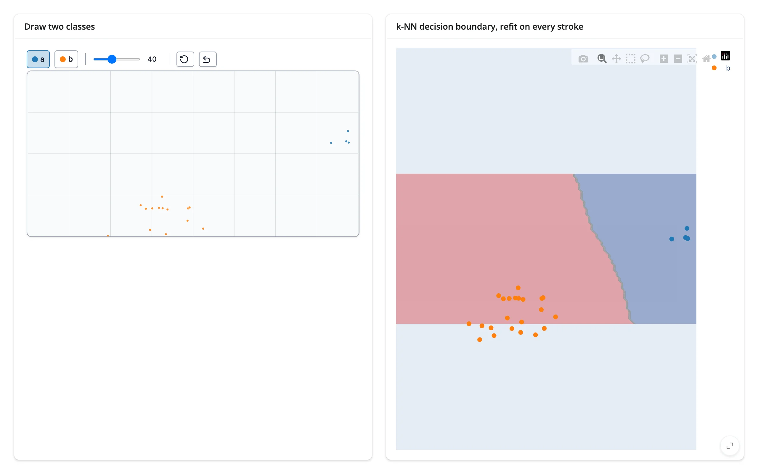
This is the headline pattern: draw two classes, and a k-NN classifier refit on every stroke paints its decision boundary right next to the canvas. See “Coordinating multiple views” below for the full code and more variations (regression, clustering, comparing distributions).
Reacting to user interaction
render_drawdata declares no reactive accessor methods – there’s no canvas.selected(). Every interaction instead goes through canvas.read("<trait>"), the general pattern documented in the render-widget guide.
Traits worth reading
| trait | returns | fires when | default rate policy |
|---|---|---|---|
data (ScatterWidget) |
list[dict] with x, y (data-space, y-up), color (hex), label ("a"-"d"), batch (int) |
a drawing batch (stroke) syncs – see the lag caveat below – or undo/reset is clicked | not rate-limited by default |
data (BarWidget) |
list[dict] with collection, value, bin, color – one entry per bin per collection, always present (defaults to 0) |
on every pointer move while dragging a bar | not rate-limited by default |
brushsize (ScatterWidget) |
int, default 40 |
dragging the brush-size slider | not rate-limited by default |
Both widgets also expose non-reactive convenience properties – .data_as_pandas, .data_as_polars, and (scatter only) .data_as_X_y – that compute once from the current trait value. They’re fine to call after you’ve already taken a dependency with .read("data") elsewhere in the same function (as in the regression example below); call one on its own and it never refires.
The one-batch sync lag
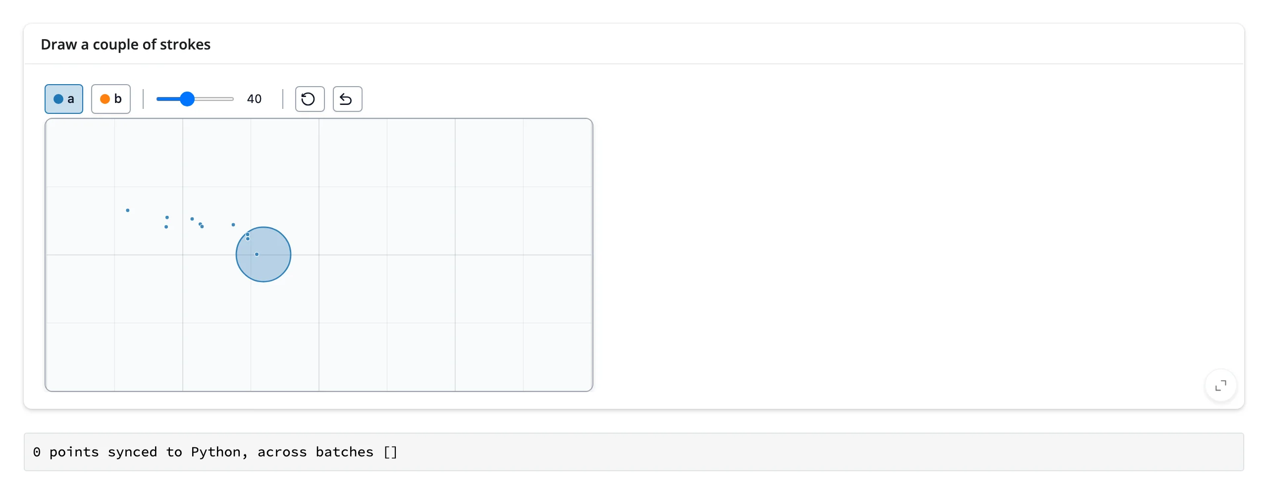
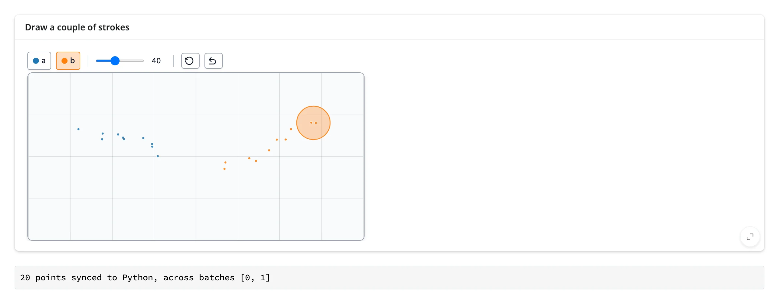
The single biggest gotcha in this guide: ScatterWidget loses track of your first drawing batch. Draw one stroke and canvas.read("data") still reports the old (possibly empty) value; draw a second stroke and Python receives all points from both. Undo and reset sync immediately, so they’re not affected.
This is an upstream drawdata bug: its frontend keeps a plain JavaScript array of points and reuses it across strokes, mutating it in place; by the time it hands the array to the model, deep-equality logic upstream sees “no change” against the model’s current (identical, pre-mutation-detection) copy and skips the sync. The next stroke’s array differs by more than just the new points, so the whole thing finally goes through. There’s no Python-side workaround – the browser genuinely hasn’t told Python about the first batch yet.
@render.code
def state():
    # Each call to .read("data") re-runs this on every *synced* change to
    # "data" -- see "Gotchas" for why the very first stroke of a session
    # doesn't show up here until a second one starts.
    data = canvas.read("data")
    batches = sorted({d["batch"] for d in data})
    return f"{len(data)} points synced to Python, across batches {batches}"
10 points drawn, 0 synced; a second stroke (10 more points) flushes both batches at once:
Rate limiting
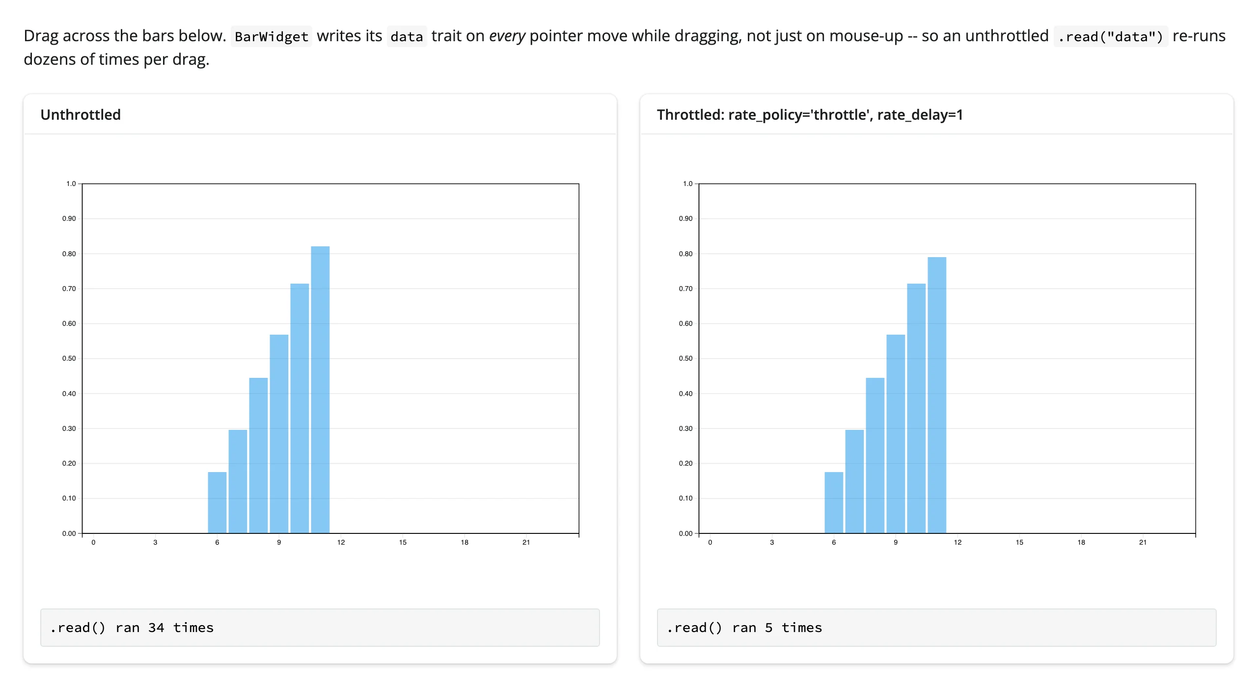
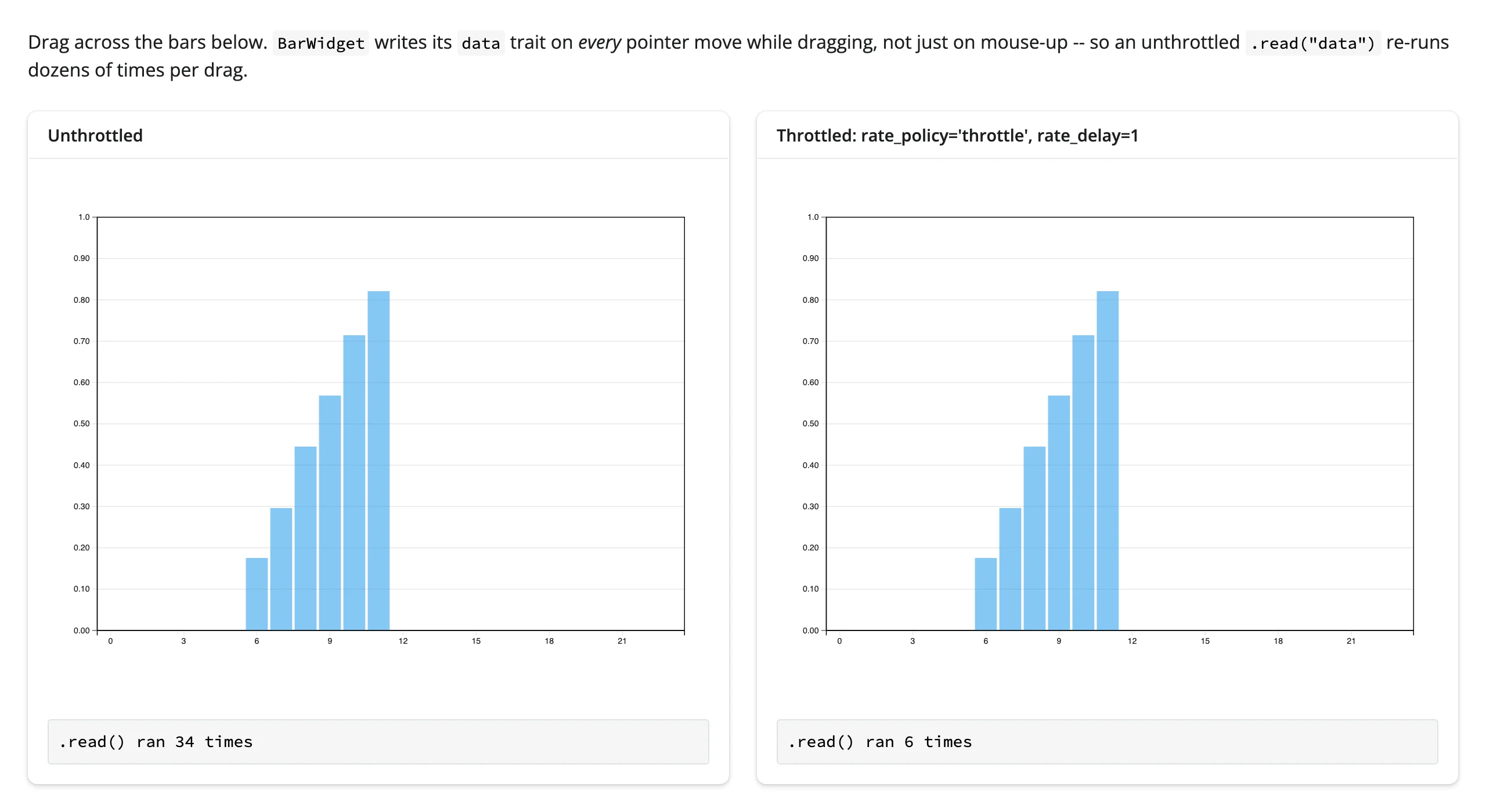
rate_policy/rate_delay on @render_drawdata rate-limit .read() for every trait on that widget, same as every other renderer’s .read() tier – there’s no default throttle unless you set one. It matters most for BarWidget, whose data trait writes on every pointer move during a drag, not just on release.
with ui.layout_columns():
    with ui.card():
        ui.card_header("Unthrottled")

        @render_drawdata
        def unthrottled():
            return BarWidget(collection_names=["dist"])

        @render.code
        def n_unthrottled():
            unthrottled.read("data")
            counts["unthrottled"] += 1
            return f".read() ran {counts['unthrottled']} times"

    with ui.card():
        ui.card_header("Throttled: rate_policy='throttle', rate_delay=1")

        @render_drawdata(rate_policy="throttle", rate_delay=1)
        def throttled():
            return BarWidget(collection_names=["dist"])

        @render.code
        def n_throttled():
            throttled.read("data")
            counts["throttled"] += 1
            return f".read() ran {counts['throttled']} times"
One continuous drag: the unthrottled reader counts every intermediate value; the throttled one catches up only after the drag pauses:
Updating the widget from Python
The two widgets behave differently here, and the difference matters for how you reset them:
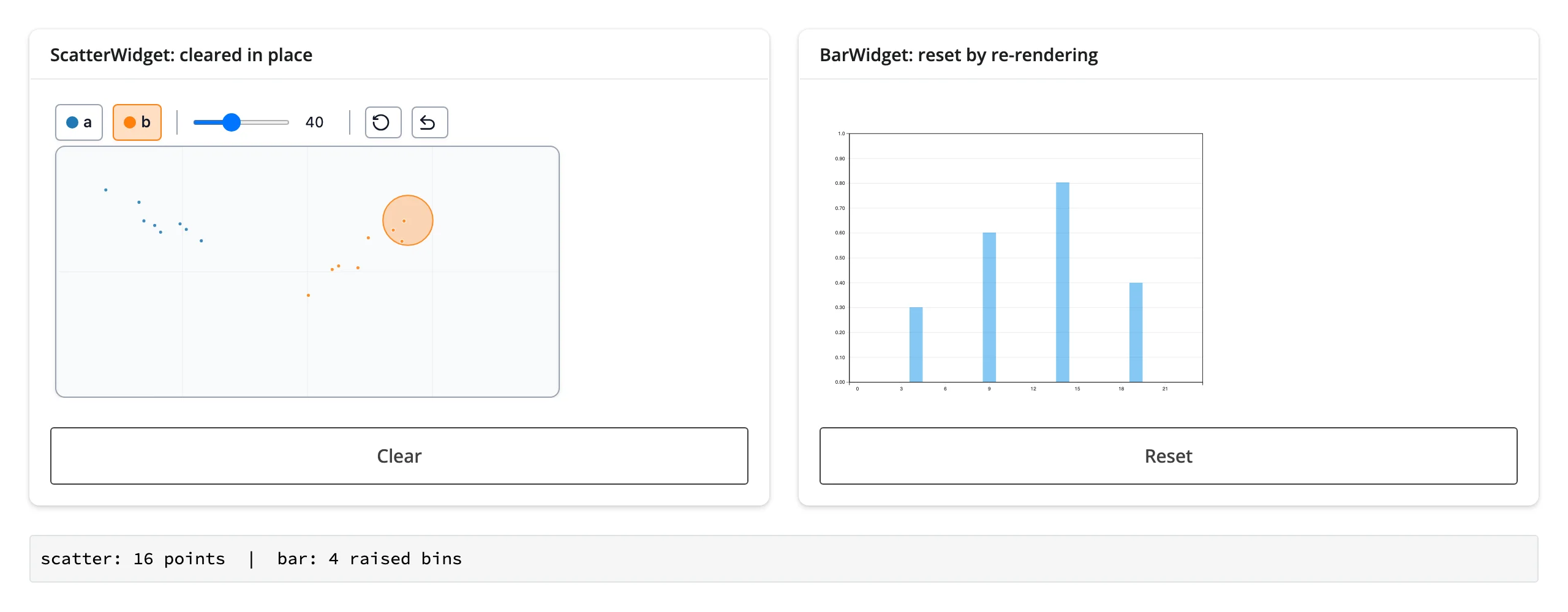
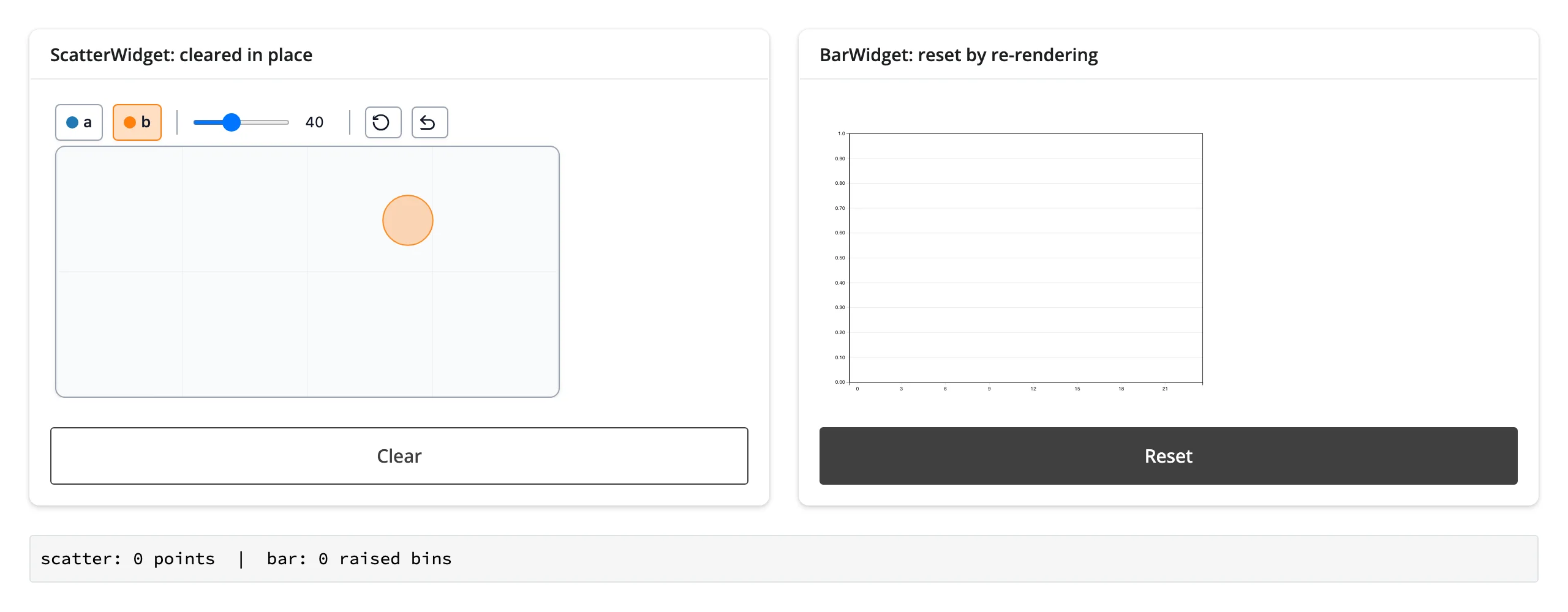
ScatterWidgetaccepts live Python-side writes. Its frontend listens forchange:data,change:brushsize,change:width, andchange:height, socanvas.widget.data = []both updates the trait and clears the browser canvas immediately – a true in-place update, no re-render.BarWidgetdoes not. Its frontend registers nochange:handlers at all, and its first render unconditionally overwrites whateverdatayou passed to the constructor with zeros. The only way to change anything about an existingBarWidget– including resetting it – is to re-render: return a newBarWidget()from the render function.
from __future__ import annotations

from drawdata import BarWidget, ScatterWidget
from shiny import reactive
from shiny.express import input, render, ui
from shinywidgets import render_drawdata

ui.page_opts(fillable=True)

# BarWidget ignores Python-side trait writes after it first renders (its
# frontend registers no `change:` handlers), so the only way to reset one is
# to re-render it. Bumping this counter -- read, but otherwise unused, inside
# the render function -- forces exactly that.
bar_generation = reactive.Value(0)

with ui.layout_columns():
    with ui.card():
        ui.card_header("ScatterWidget: cleared in place")

        @render_drawdata
        def canvas():
            return ScatterWidget(width=800, height=400, n_classes=2)

        ui.input_action_button("clear_canvas", "Clear")

    with ui.card():
        ui.card_header("BarWidget: reset by re-rendering")

        @render_drawdata
        def hist():
            bar_generation()
            return BarWidget(collection_names=["dist"])

        ui.input_action_button("reset_hist", "Reset")


@render.code
def counts():
    s = canvas.read("data")
    b = [d for d in hist.read("data") if d["value"] != 0]
    return f"scatter: {len(s)} points  |  bar: {len(b)} raised bins"


@reactive.effect
@reactive.event(input.clear_canvas)
def _clear_canvas():
    # ScatterWidget *does* have a change:data handler, so this both updates
    # the Python-side trait and clears the browser canvas immediately.
    canvas.widget.data = []


@reactive.effect
@reactive.event(input.reset_hist)
def _reset_hist():
    bar_generation.set(bar_generation() + 1)
Both drawings cleared with one click each – the scatter in place, the bar by re-render:
Coordinating multiple views
These are the patterns worth stealing. Each draws into a ScatterWidget or BarWidget and feeds a second, independent output that updates on every synced batch.
A live classifier decision boundary (plotly)
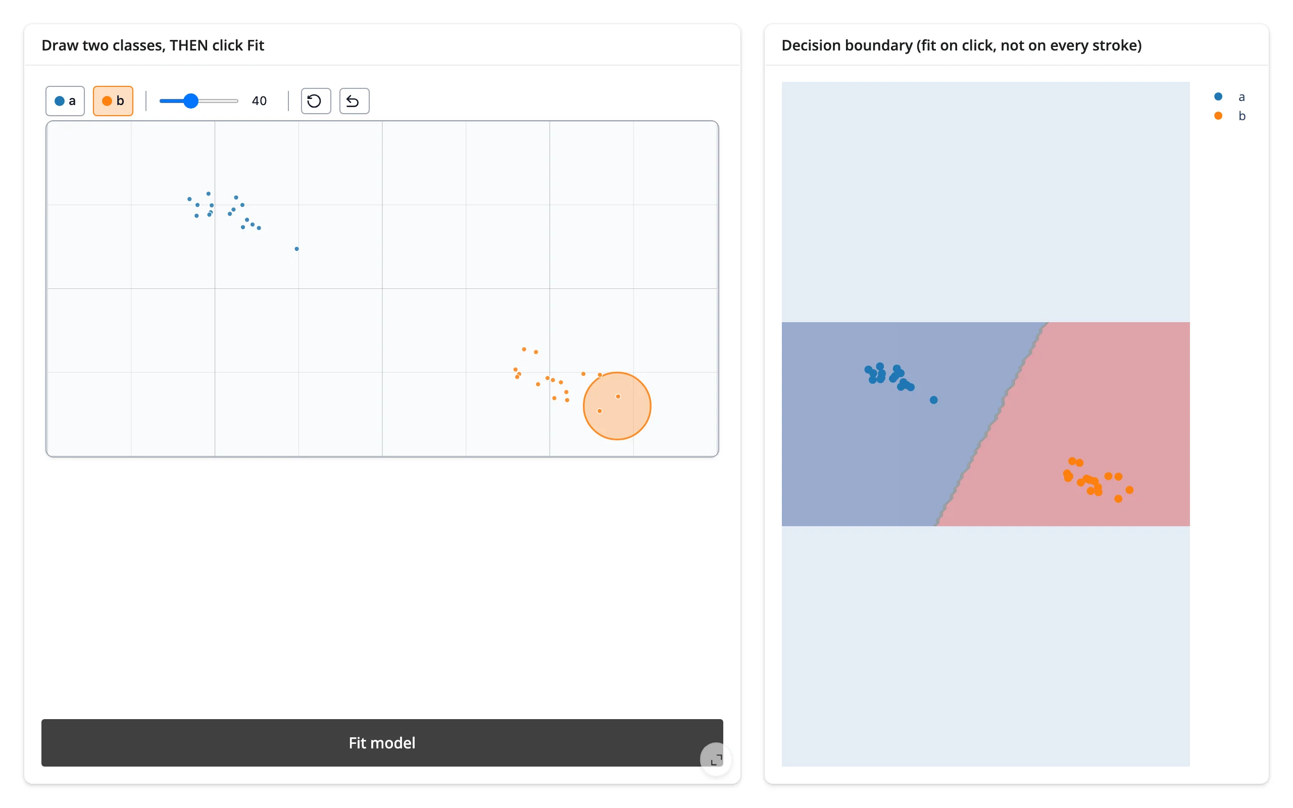
Draw two classes; a k-NN classifier refits on every stroke and plotly draws its decision regions underneath the points. scaleanchor="x" on the y-axis keeps the plot’s aspect ratio matched to the canvas, so the boundary lines up visually with where you drew.
        @render_plotly
        def boundary():
            df = pd.DataFrame(canvas.read("data"))
            fig = go.Figure()
            fig.update_xaxes(range=[0, W], visible=False)
            fig.update_yaxes(range=[0, H], visible=False, scaleanchor="x")
            fig.update_layout(margin=dict(l=0, r=0, t=0, b=0))
            if df.empty or df["label"].nunique() < 2:
                fig.add_annotation(
                    text="draw points of both classes",
                    x=W / 2,
                    y=H / 2,
                    showarrow=False,
                )
                return fig

            X = df[["x", "y"]].to_numpy()
            y = df["label"].to_numpy()
            clf = KNeighborsClassifier(n_neighbors=min(5, len(X))).fit(X, y)

            gx, gy = np.meshgrid(np.linspace(0, W, 120), np.linspace(0, H, 60))
            grid = np.c_[gx.ravel(), gy.ravel()]
            _, pred_idx = np.unique(clf.predict(grid), return_inverse=True)
            fig.add_contour(
                x=gx[0],
                y=gy[:, 0],
                z=pred_idx.reshape(gx.shape),
                showscale=False,
                opacity=0.35,
                colorscale="Portland",
            )
            for label, group in df.groupby("label"):
                fig.add_scatter(
                    x=group["x"],
                    y=group["y"],
                    mode="markers",
                    marker=dict(color=group["color"].iloc[0], size=8),
                    name=label,
                )
            return fig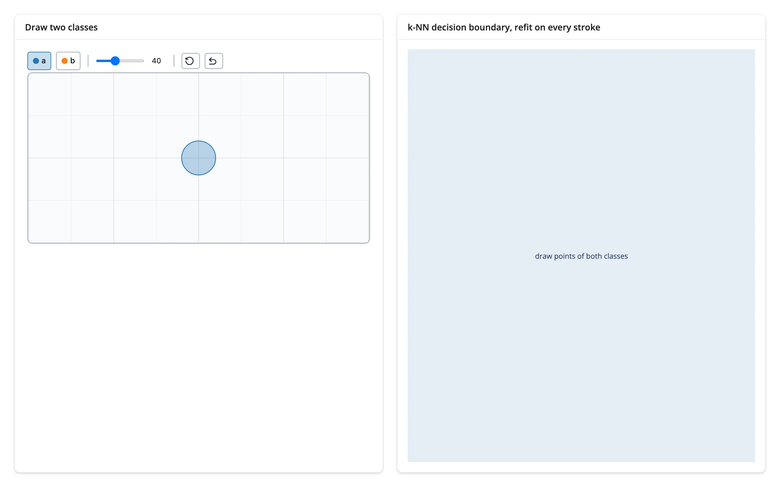
The gallery template below wraps this pattern with a neighbor-count slider and a clear button – start there if you want a polished version to adapt.
Fit on demand, not on every stroke
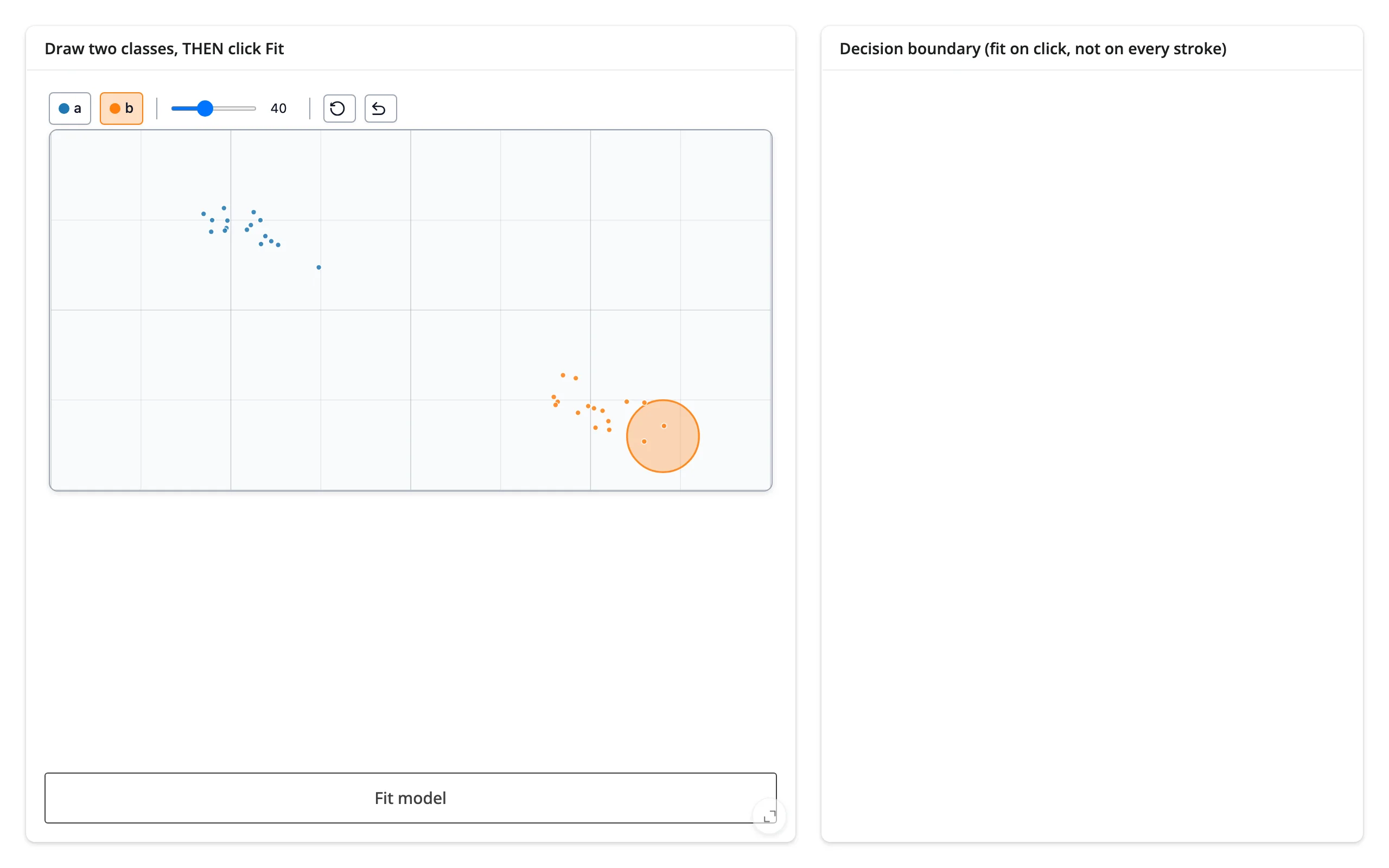
The classifier above refits on every synced batch – fine for k-NN, but a heavier model (a grid search, a GPU model, a slow custom fit) would make every stroke pause the UI. Gate the read behind a button instead with @reactive.event(input.fit): nothing reads canvas.read("data") until the user clicks “Fit model”, but because a synced trait holds whatever the browser last reported the moment the widget renders – not just from the output’s first read – every point drawn before that click is still there when it finally runs.
        @render_plotly
        @reactive.event(input.fit)
        def boundary():
            # Nothing reads "data" until this click -- not a warm-up read,
            # not a visible output, nothing -- but every point drawn before
            # the click is still here: a synced trait holds the latest value
            # the moment the widget renders, whether or not anything has
            # read it yet. That's what makes "fit only when asked" safe
            # instead of needing a k-NN refit on every single stroke.
            df = pd.DataFrame(canvas.read("data"))
Draw both classes first – the right panel stays completely empty, because nothing has read the data yet. Click “Fit model” and the whole drawing, both classes, shows up at once:
A live regression fit (matplotlib)
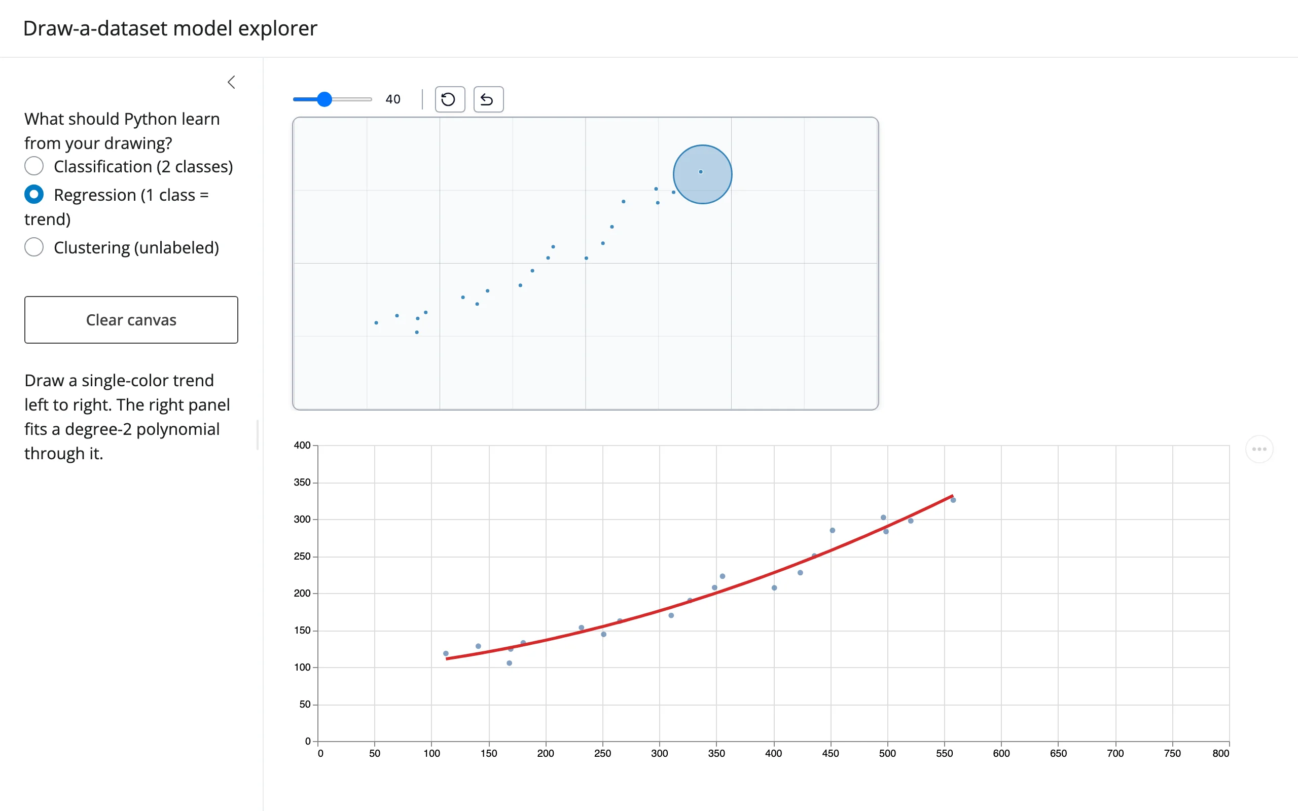
With n_classes=1, every point is the same color; drawdata’s own data_as_X_y property then reinterprets the drawing as regression data (X = the x-coordinates, y = the y-coordinates) instead of classification data. Draw a trend left to right and a quadratic curve refits underneath it.
        @render_matplotlib
        def fit():
            # A dependency on "data" also covers data_as_X_y, computed from
            # the same trait; with one color drawn, it returns (X, y) for
            # regression instead of (X, hex colors) for classification.
            canvas.read("data")
            X, y = canvas.widget.data_as_X_y

            fig, ax = plt.subplots(figsize=(5, 2.5))
            ax.set_xlim(0, W)
            ax.set_ylim(0, H)
            if len(X) < 3:
                ax.text(
                    W / 2, H / 2, "draw at least 3 points", ha="center", color="grey"
                )
                return fig
            x = X.ravel()
            coeffs = np.polyfit(x, y, deg=2)
            xs = np.linspace(x.min(), x.max(), 100)
            ax.scatter(x, y, s=12, color="#1f77b4")
            ax.plot(xs, np.polyval(coeffs, xs), color="#d62728", linewidth=2)
            return fig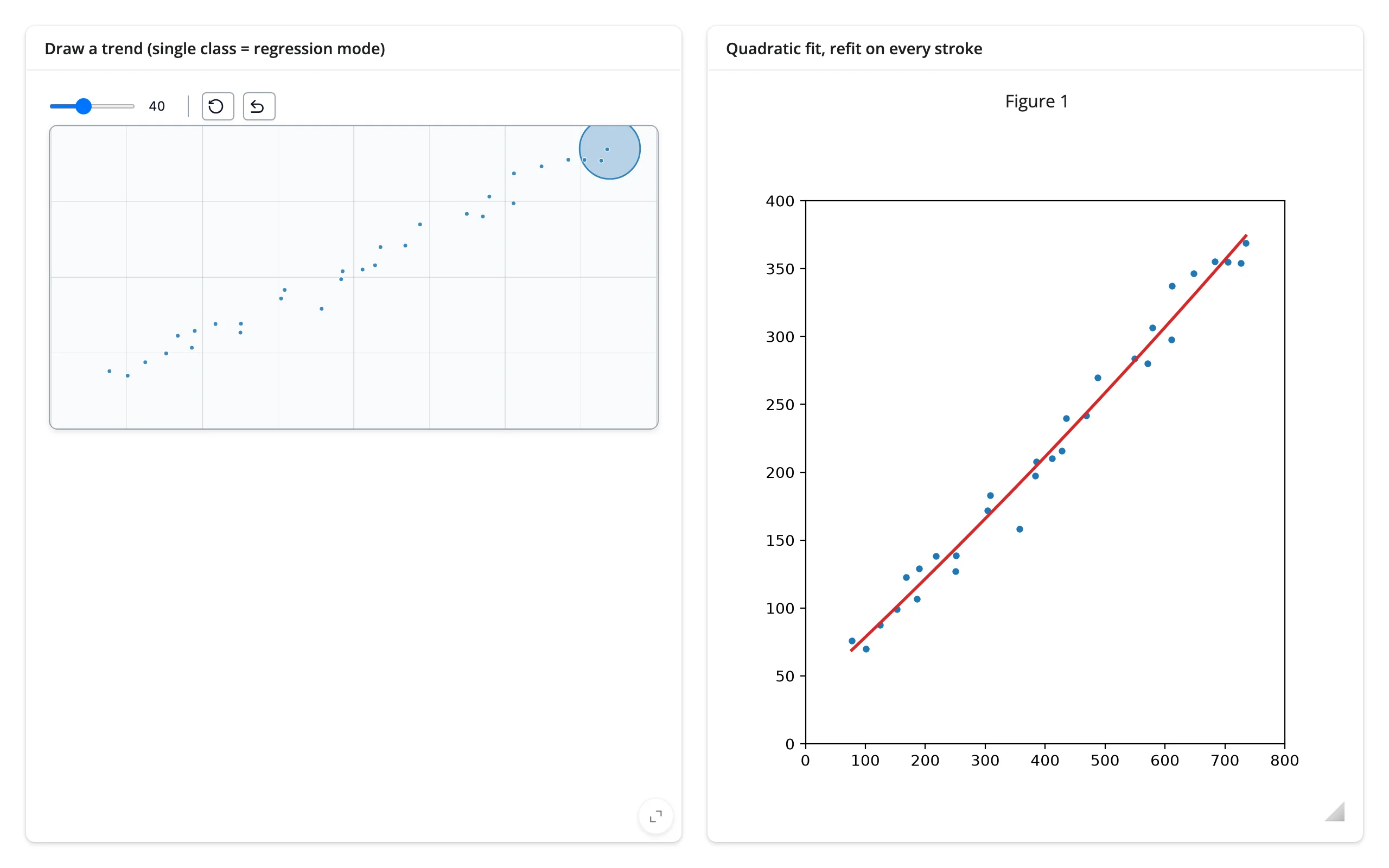
Comparing two sculpted distributions (altair)
BarWidget’s default collection_names (["collection1", "collection2"]) gives you a button to switch which distribution you’re currently sculpting – useful for drawing two distributions to compare side by side. Altair redraws both, overlaid with opacity, from the same data trait every other example uses.
        @render_altair
        def overlay():
            df = pd.DataFrame(hist.read("data"))
            chart = (
                alt.Chart(df)
                .mark_bar(opacity=0.7)
                .encode(
                    x=alt.X("bin:O", title=None),
                    y=alt.Y("value:Q", title=None, stack=None),
                    color=alt.Color("collection:N", legend=alt.Legend(title=None)),
                )
            )
            return chart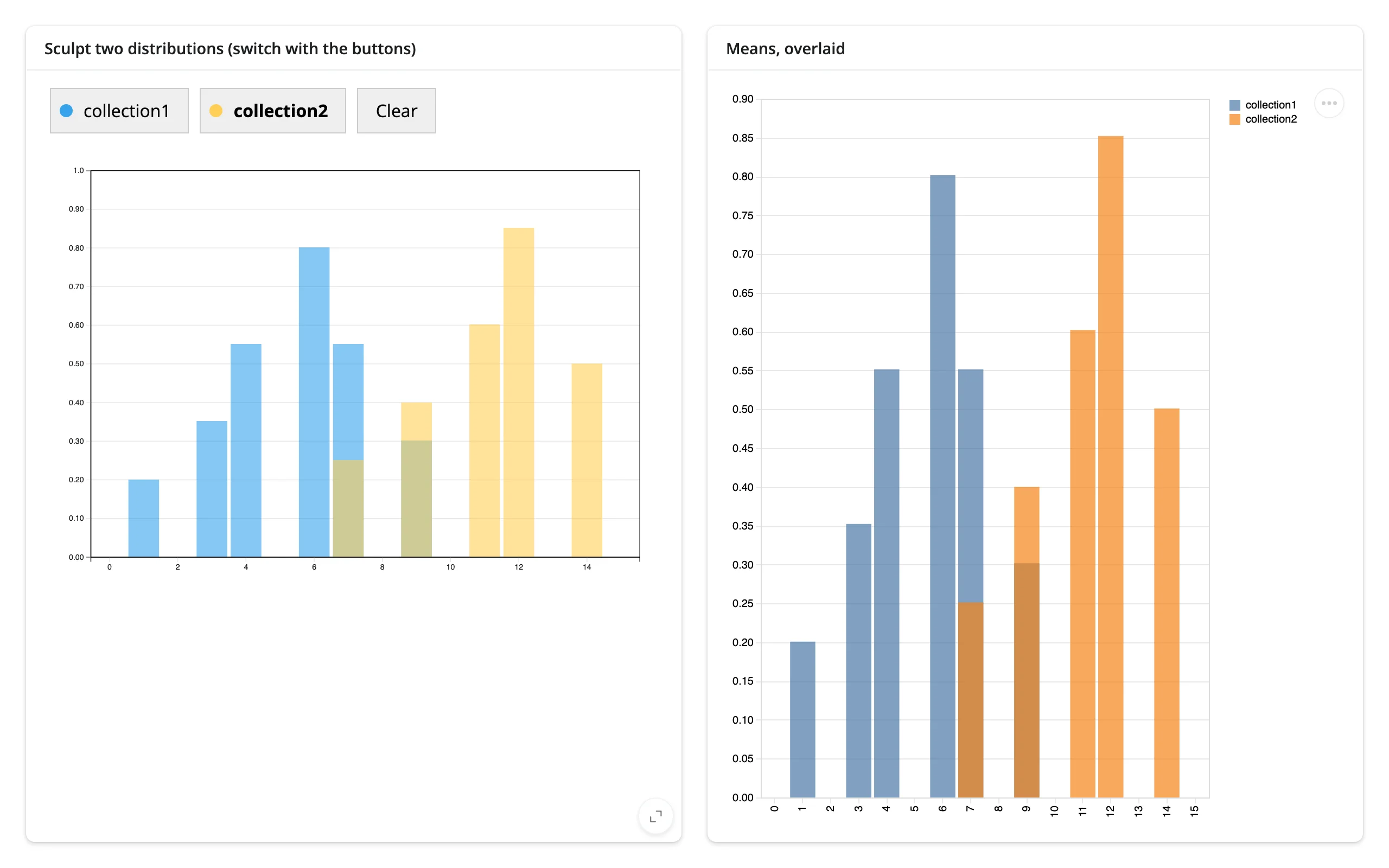
Live clustering (altair)
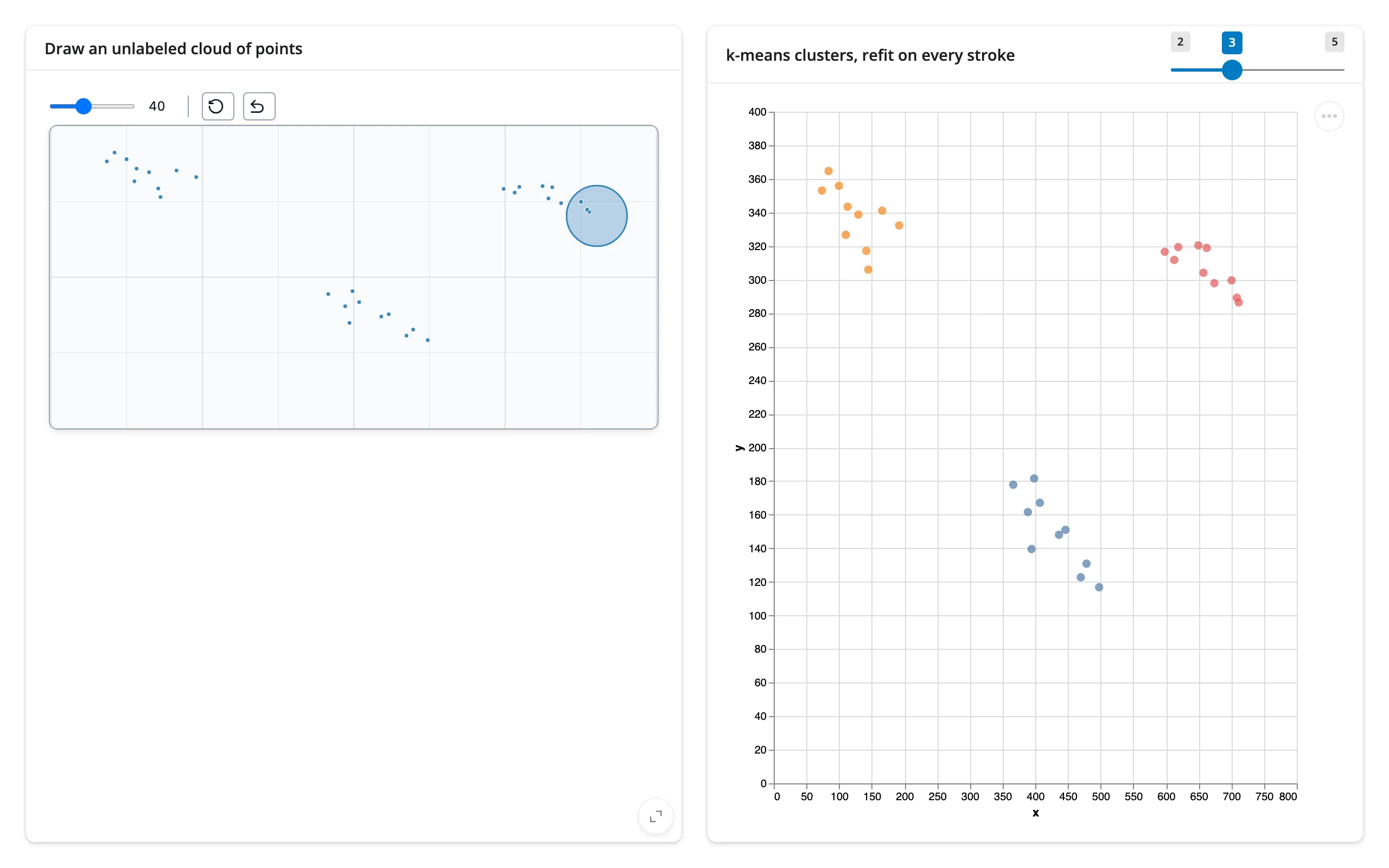
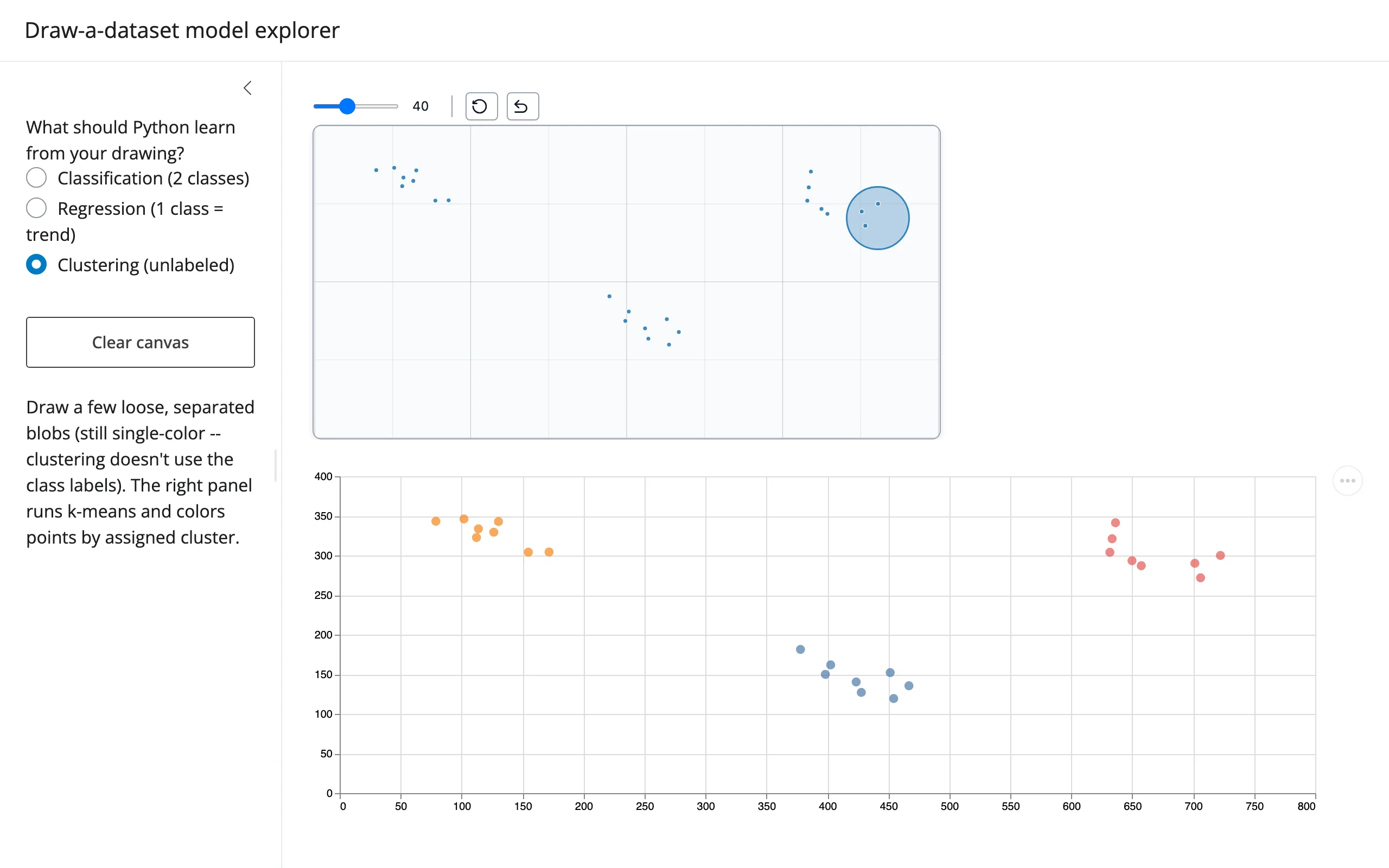
Clustering doesn’t need labels at all: draw a single-color cloud of points (n_classes=1) and k-means (k from a slider) assigns and colors clusters live.
        @render_altair
        def clusters():
            df = pd.DataFrame(canvas.read("data"))
            base = (
                alt.Chart()
                .mark_point()
                .encode(
                    x=alt.X("x:Q", scale=alt.Scale(domain=[0, W])),
                    y=alt.Y("y:Q", scale=alt.Scale(domain=[0, H])),
                )
            )
            if len(df) < input.k():
                return base
            labels = KMeans(n_clusters=input.k(), n_init=5, random_state=0).fit_predict(
                df[["x", "y"]]
            )
            df["cluster"] = [str(c) for c in labels]
            return (
                alt.Chart(df)
                .mark_point(filled=True, size=60)
                .encode(
                    x=alt.X("x:Q", scale=alt.Scale(domain=[0, W])),
                    y=alt.Y("y:Q", scale=alt.Scale(domain=[0, H])),
                    color=alt.Color("cluster:N", legend=None),
                )
            )
Pairs with: plotly (contour fills for decision regions), matplotlib (quick static fits), altair (categorical overlays and grouped bars).
Layout and sizing
Both widgets have an intrinsic pixel size from their constructor’s width/height traits (ScatterWidget defaults to 800x400, BarWidget to 800x550) – but that size is really the data coordinate space the drawing is stored in, not a fixed display size. Upstream, both widgets cap their on-screen display at that same pixel size; render_drawdata lifts the cap so the widget instead fills the output’s width, scaling its display while preserving the trait-defined aspect ratio. In an output with an explicit height (output_widget(height=...), or any fill layout), the chart is also constrained to fit that height. This is the one real shinywidgets-side fix in this renderer – without it, BarWidget’s default 550px-tall chart gets clipped at the generic 400px flex basis most other outputs use.
Practical implications: - Pick the constructor’s width/height for the coordinate range and aspect ratio you want to draw in, not for a target pixel size – ScatterWidget(width=1000, height=500) draws in a 2:1 box no matter how large or small the rendered output ends up. - BarWidget’s bars are keyed by index (bin), independent of display size, so sizing never affects how a drawn distribution reads back. - Use ui.card(full_screen=True) and fill=True as you would for any other widget; nothing about drawdata’s sizing behavior requires special handling in the UI.
Gotchas and limitations
Verified on current main (drawdata 0.5.2):
ScatterWidget’s first drawing batch doesn’t sync until a second one starts – see “The one-batch sync lag” above. This is the thing you will hit first; don’t build a flow that depends on seeing the user’s very first stroke in isolation.BarWidgetignores every Python-side trait write after its first render, including thedatayou pass to its constructor (which gets silently overwritten with zeros on mount). Treat a renderedBarWidgetas browser-driven only; re-render to change anything, including resetting it.BarWidget’s defaultcollection_namesis["collection1", "collection2"], not a single distribution – you get a two-way switcher and a “Clear” button out of the box. Pass a one-element list (collection_names=["dist"]) for a single plain distribution with no extra controls. Also avoid putting twoBarWidgets on the same page: clicking one’s collection buttons can affect the other’s active collection (both attach the same globalbutton.controlclick listener).data_as_X_yreports hex color codes asyfor classification, not the"a"/"b"/"c"/"d"labels – usedata_as_pandas["label"](or build the array from.read("data")yourself, as the classifier example above does) if you need the actual class names.- One harmless console error per
ScatterWidgetrender:<svg> attribute height: Expected length, "auto". It’s an invalid attribute upstream sets (the real sizing comes from CSSaspect-ratio); it shows up in Jupyter too and has no visible effect. .data_as_pandas/.data_as_polars/.data_as_X_yare plain property reads, not reactive. Call them only after a.read("data")elsewhere in the same function; on their own they compute once from whatever the trait held at that moment and never refire.
Gallery candidates
Template: classifier playground
gallery/template_classifier_playground.py – the classifier pattern above, cleaned up with a neighbor-count slider and a clear button. ~65 lines; swap KNeighborsClassifier for any other scikit-learn classifier to adapt it.
uv run --with scikit-learn shiny run docs/widget-guides/drawdata/gallery/template_classifier_playground.py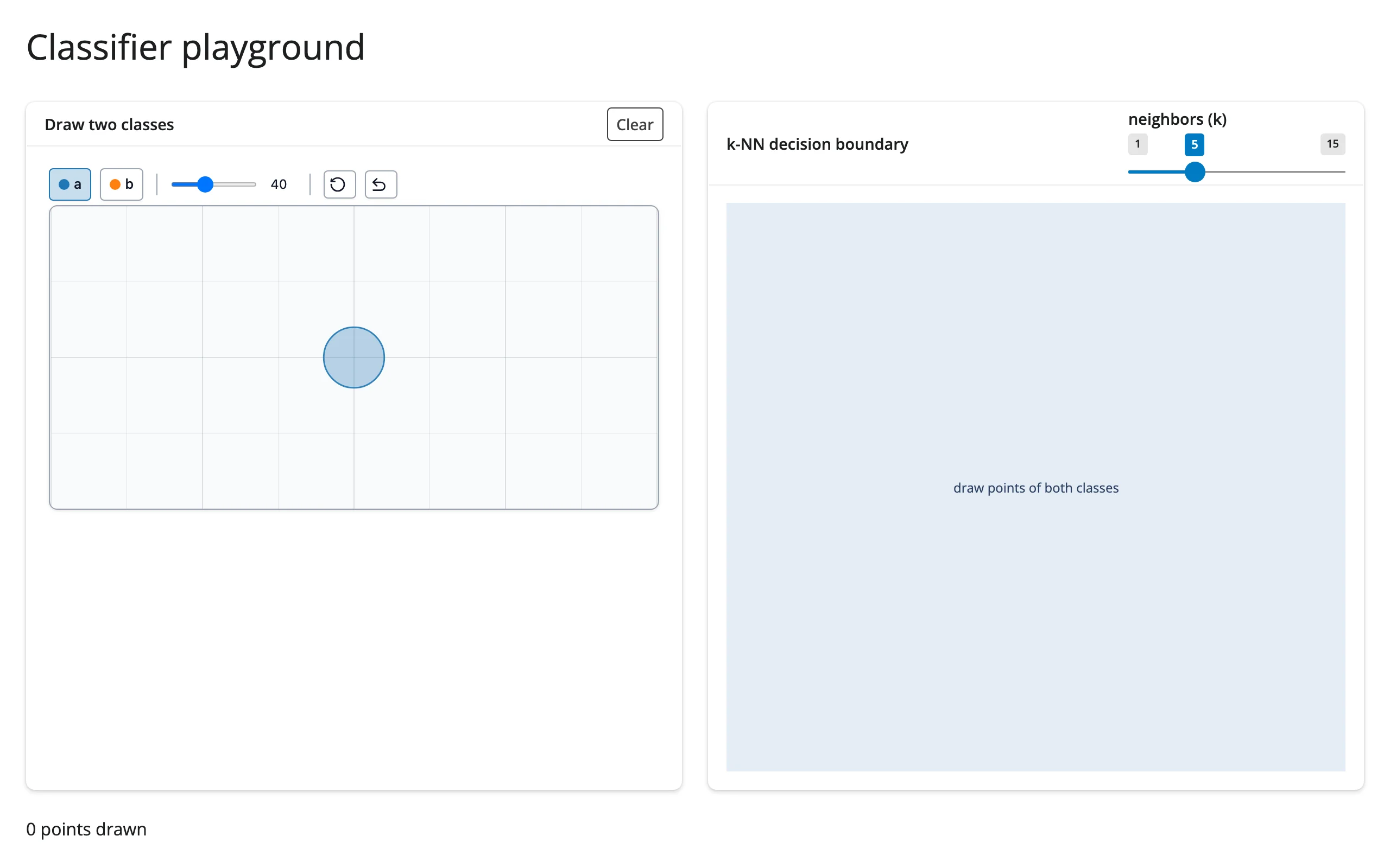
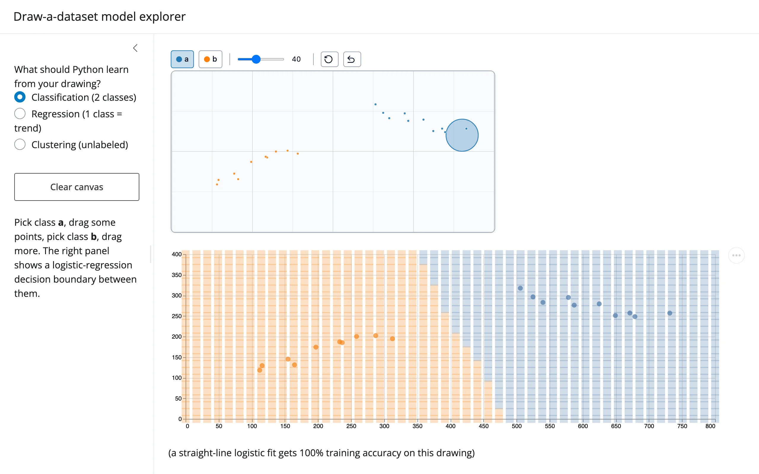
Showcase: draw-a-dataset model explorer
gallery/showcase_model_explorer.py – one canvas, three ML tasks (classification, regression, clustering) picked with a sidebar radio button. Switching tasks re-renders the canvas with the right n_classes for that task and clears the drawing; a “Clear canvas” button does the same on demand.
uv run --with scikit-learn shiny run docs/widget-guides/drawdata/gallery/showcase_model_explorer.py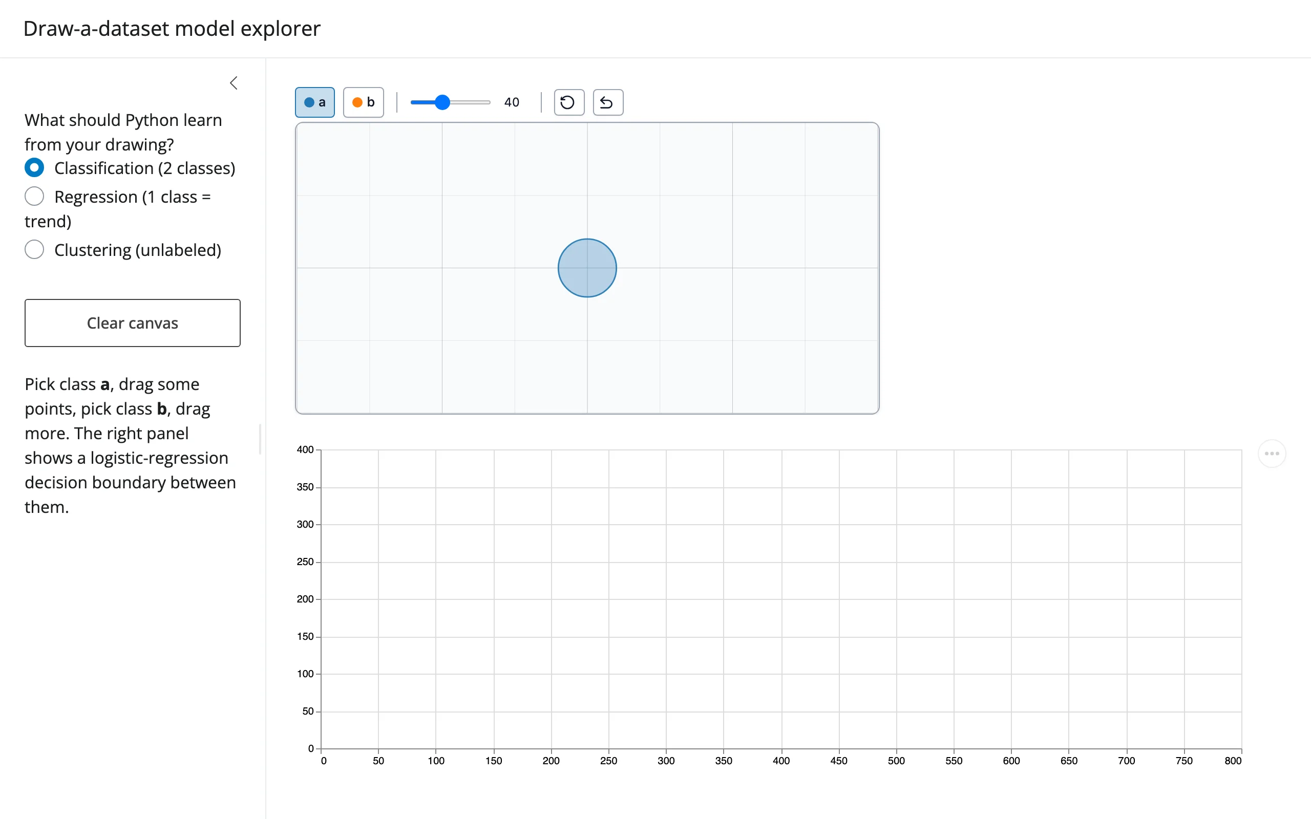
Learn more
- drawdata docs / live demo
- drawdata on GitHub
- render-widget guide – the general
.read()pattern used throughout this guide - plotly, matplotlib, altair – the model views paired with drawdata above
- ipycanvas – for free-form drawing/annotation rather than point-and-bar datasets