Bokeh

Build plots out of live Python objects – selections, ranges, and widget values sync both ways, with no Bokeh server required.

Bokeh is a Python plotting library built and maintained by Anaconda. Unlike most plotting libraries, a Bokeh plot isn’t a static picture that gets redrawn – it’s a tree of live Python objects (a figure, its ColumnDataSources, axes, tools, widgets) that stay connected to the browser. Normally that connection requires running a bokeh serve process. shinywidgets recreates it inside a Shiny app instead, through jupyter_bokeh, so Bokeh’s full Python object model – selections, ranges, events, even Bokeh’s own Slider/Select/DataTable widgets – works without a separate server.

@render_bokeh accepts a bokeh.plotting.figure, a layout (row, column, gridplot), any other LayoutDOM (a Div, a Bokeh widget), or a jupyter_bokeh.BokehModel you built yourself. It fills its card by default: a bare figure() gets sizing_mode="stretch_both" unless you give it a width, height, sizing_mode, or aspect_ratio, in which case Bokeh’s own sizing takes over. BokehJS loads automatically, including for outputs created dynamically inside @render.ui.

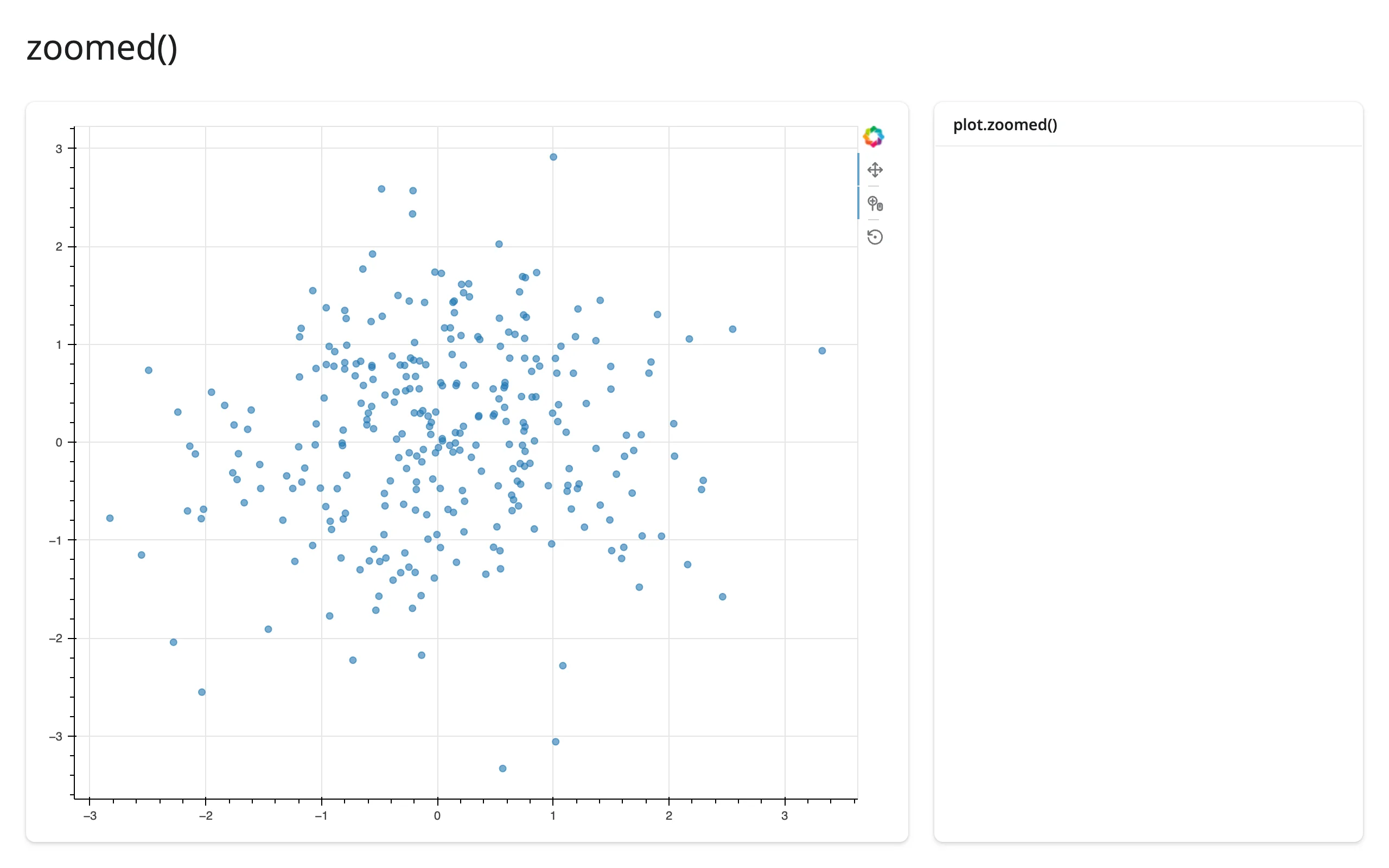
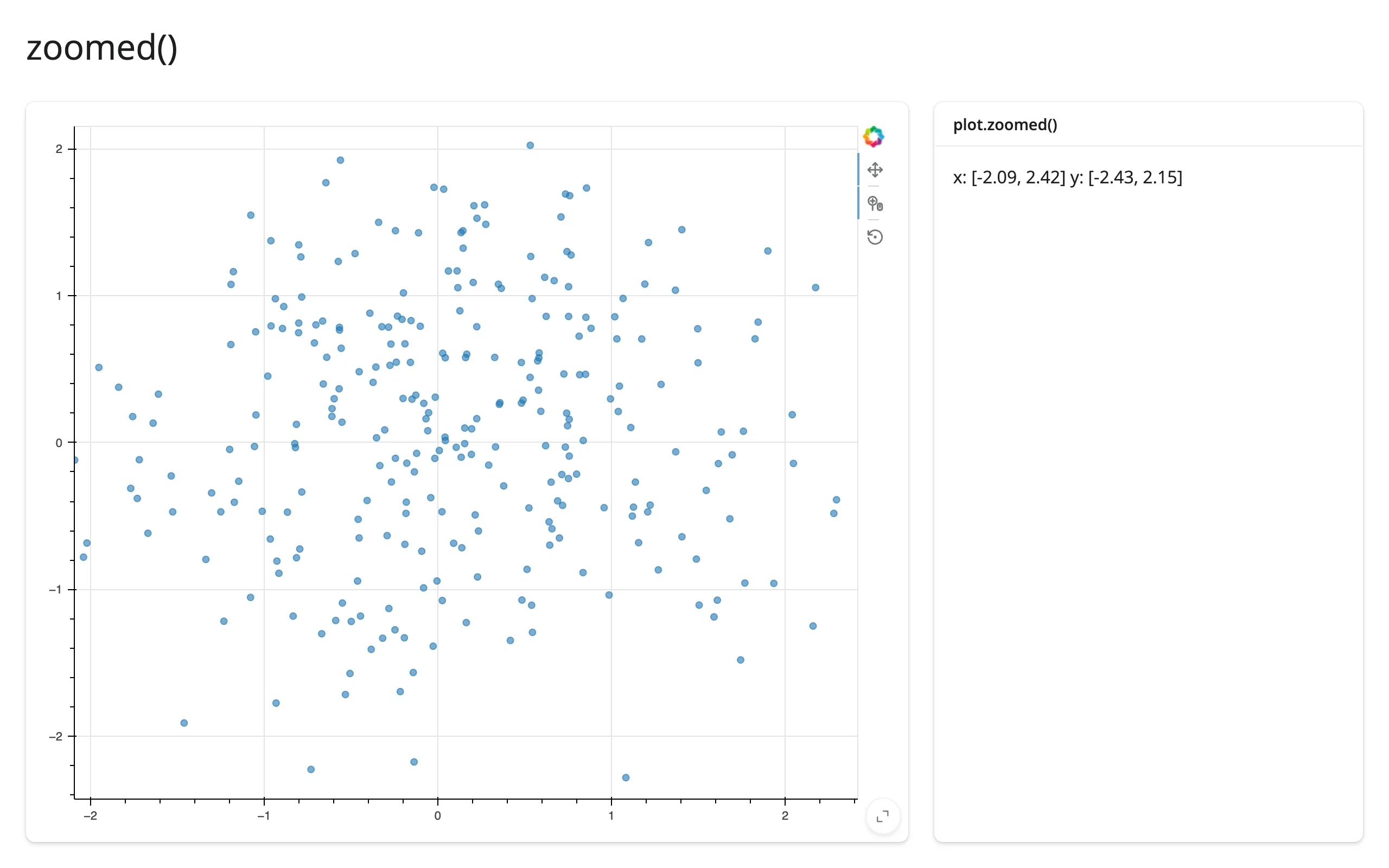
The four accessors below (selected(), selected_rows(), tapped(), zoomed()) read the single most common things apps need from a plot: its selection, its last click, and its current view. For anything else, Bokeh’s own on_change()/on_event() callbacks work directly inside a reactive context – which is also how you’d reach Bokeh’s own widgets (Slider, Select, DataTable) or an editing tool like PointDrawTool.

Choose Bokeh when you want linked views that update in the browser with no round trip, Python callbacks on any part of the plot (not just a curated set of events), editable plots, or you’re porting code written for bokeh serve. Choose plotly for more chart types and smoother 3D; choose altair for a declarative grammar of selections; choose holoviews or panel (both covered in their own guides) if you’re already building on top of those – they render through Bokeh under the hood but don’t get accessors.

Installation

pip install 'shinywidgets[bokeh]'

That installs bokeh and jupyter_bokeh>=4.1. The version floor matters: jupyter_bokeh 4.1 serves its JavaScript locally, so apps work offline; earlier versions fall back to a CDN. Nothing else to configure – output_widget() (for Shiny Core) or a bare @render_bokeh function (Shiny Express) is all the UI needs.

Quick start

A figure() with no explicit size fills its card:

examples/01_quickstart.py19 lines

# Uses bokeh's own sample-data package (downloaded on first use):
#   pip install bokeh_sampledata
from bokeh.plotting import figure
from bokeh.sampledata.autompg import autompg as df
from shiny.express import ui
from shinywidgets import render_bokeh

ui.page_opts(title="Bokeh quickstart", fillable=True)

with ui.card(full_screen=True):
    ui.card_header("Fuel economy vs. weight (1970-82 cars)")

    @render_bokeh
    def plot():
        p = figure(title="EPA mileage drops as cars get heavier")
        p.xaxis.axis_label = "weight (lbs)"
        p.yaxis.axis_label = "mpg"
        p.scatter(df.weight, df.mpg, size=8, alpha=0.6)
        return p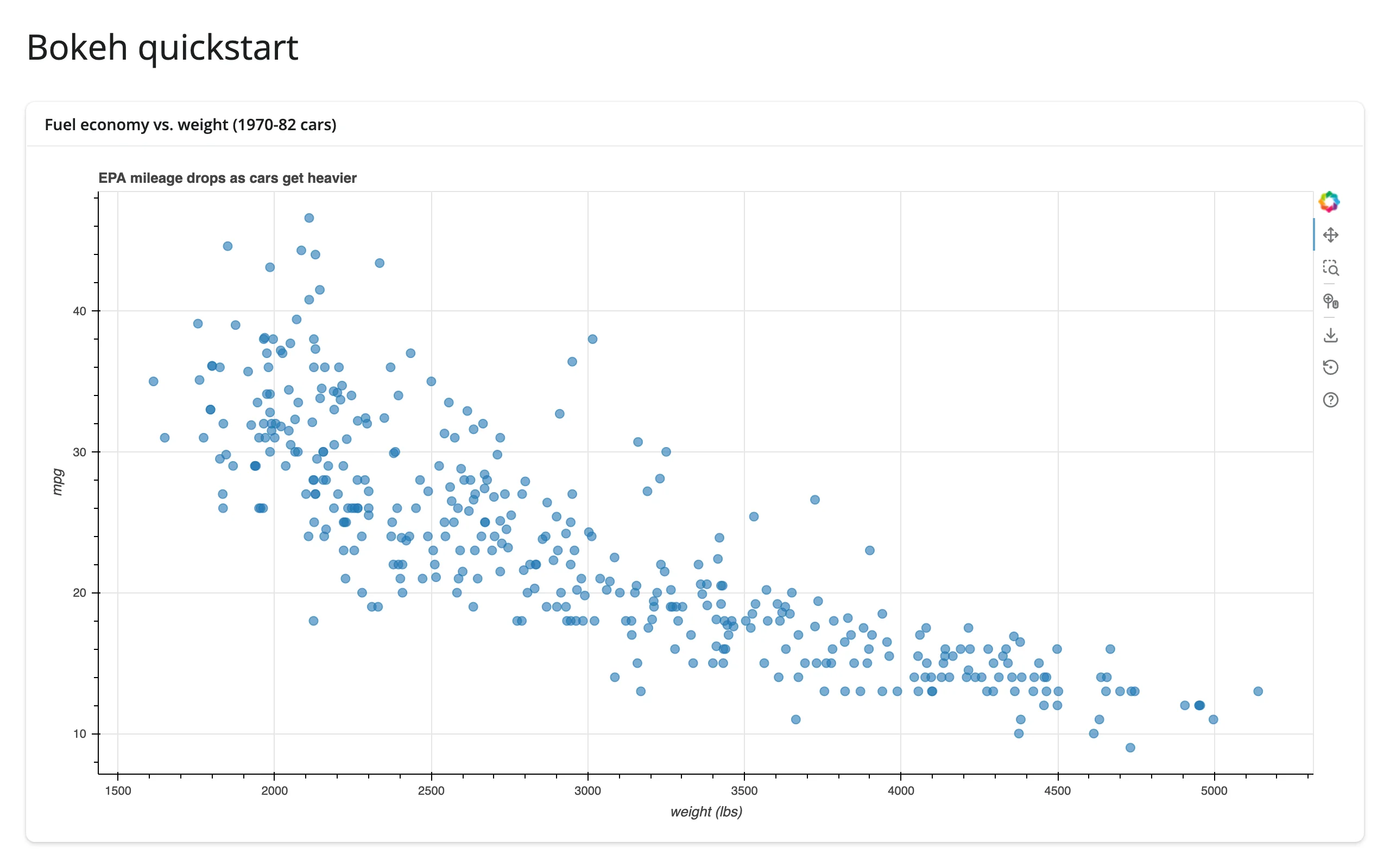

What you can build

Layouts fill their card too

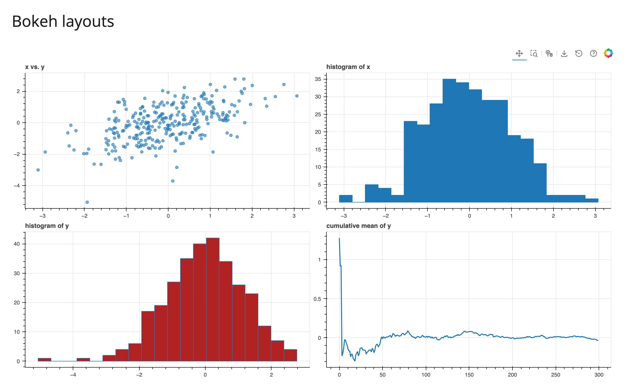
row, column, and gridplot all participate in filling, as long as both the layout and its children ask for it. A 2x2 gridplot of stretch_both figures divides the available space evenly:

examples/02_layouts.py32 lines

import numpy as np
from bokeh.layouts import gridplot
from bokeh.plotting import figure
from shiny.express import ui
from shinywidgets import render_bokeh

ui.page_opts(title="Bokeh layouts", fillable=True)

rng = np.random.default_rng(0)
x = rng.normal(size=300)
y = x * 0.6 + rng.normal(size=300)


@render_bokeh
def grid():
    scatter = figure(title="x vs. y", sizing_mode="stretch_both")
    scatter.scatter(x, y, size=6, alpha=0.6)

    hx, ex = np.histogram(x, bins=20)
    hist_x = figure(title="histogram of x", sizing_mode="stretch_both")
    hist_x.quad(top=hx, bottom=0, left=ex[:-1], right=ex[1:])

    hy, ey = np.histogram(y, bins=20)
    hist_y = figure(title="histogram of y", sizing_mode="stretch_both")
    hist_y.quad(top=hy, bottom=0, left=ey[:-1], right=ey[1:], fill_color="firebrick")

    cum = figure(title="cumulative mean of y", sizing_mode="stretch_both")
    cum.line(np.arange(len(y)), np.cumsum(y) / np.arange(1, len(y) + 1), line_width=2)

    return gridplot(
        [[scatter, hist_x], [hist_y, cum]], sizing_mode="stretch_both"
    )

Bokeh’s own widgets, wired up with ordinary Python callbacks

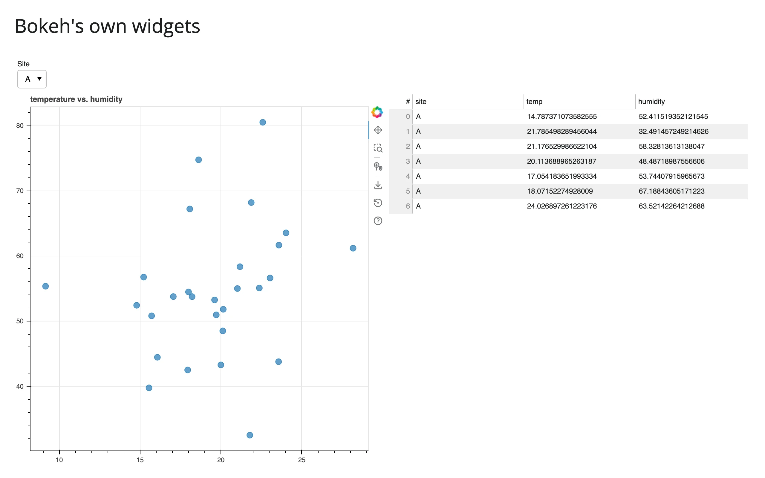
Bokeh ships Slider, Select, DataTable, and more. Their on_change/on_event callbacks run inside Shiny’s reactive machinery, so a callback that mutates a ColumnDataSource updates every view that reads it – here, a Select filters both a scatter plot and a DataTable sharing one source:

examples/03_bokeh_widgets.py43 lines

import numpy as np
from bokeh.layouts import column, row
from bokeh.models import ColumnDataSource, DataTable, Select, TableColumn
from bokeh.plotting import figure
from shiny.express import ui
from shinywidgets import render_bokeh

ui.page_opts(title="Bokeh's own widgets", fillable=True)

rng = np.random.default_rng(1)
data = {
    "temp": rng.normal(20, 4, 90),
    "humidity": rng.normal(55, 10, 90),
    "site": rng.choice(["A", "B", "C"], size=90),
}


@render_bokeh
def dashboard():
    src = ColumnDataSource(data)
    view = ColumnDataSource(data)

    p = figure(title="temperature vs. humidity", sizing_mode="stretch_both")
    p.scatter("temp", "humidity", source=view, size=10, alpha=0.7)

    table = DataTable(
        source=view,
        columns=[TableColumn(field=c) for c in ("site", "temp", "humidity")],
        height=200,
    )

    picker = Select(title="Site", value="All", options=["All", "A", "B", "C"])

    def filter_site(attr, old, new):
        if new == "All":
            view.data = dict(src.data)
        else:
            mask = src.data["site"] == new
            view.data = {k: np.asarray(v)[mask] for k, v in src.data.items()}

    picker.on_change("value", filter_site)

    return column(picker, row(p, table, sizing_mode="stretch_both"), sizing_mode="stretch_both")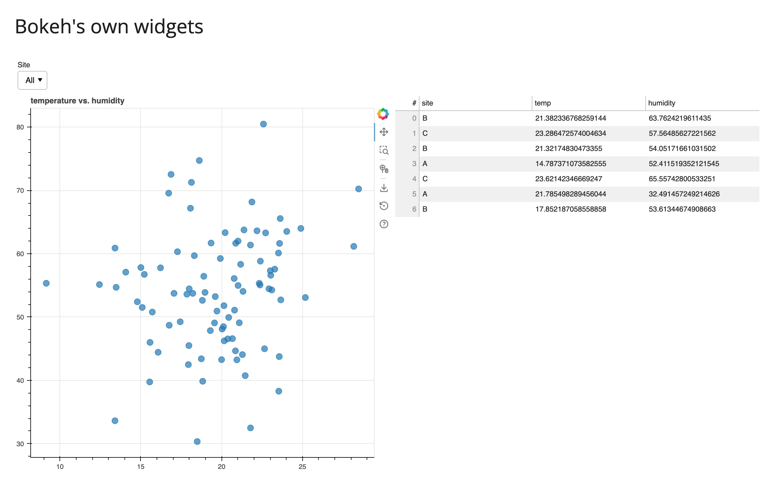

bokeh widgets before bokeh widgets after

Editable plots

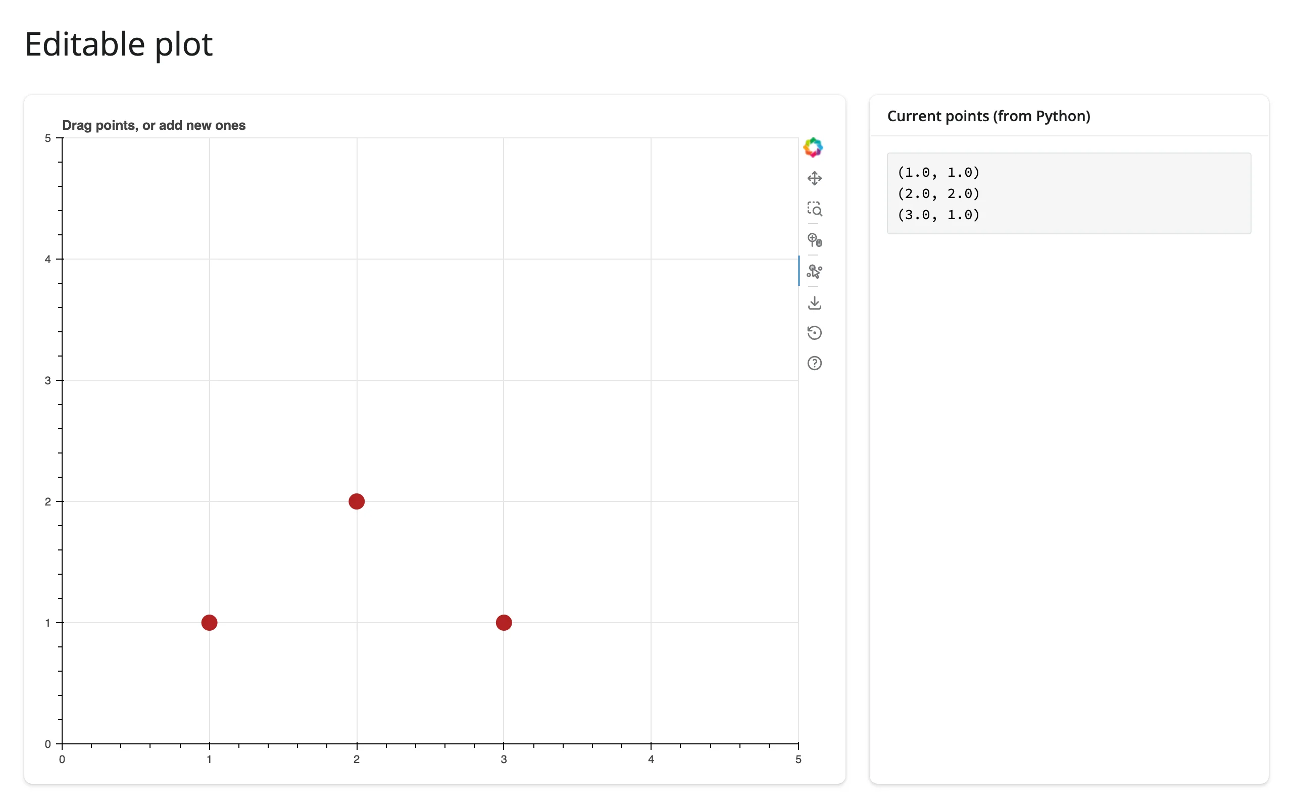
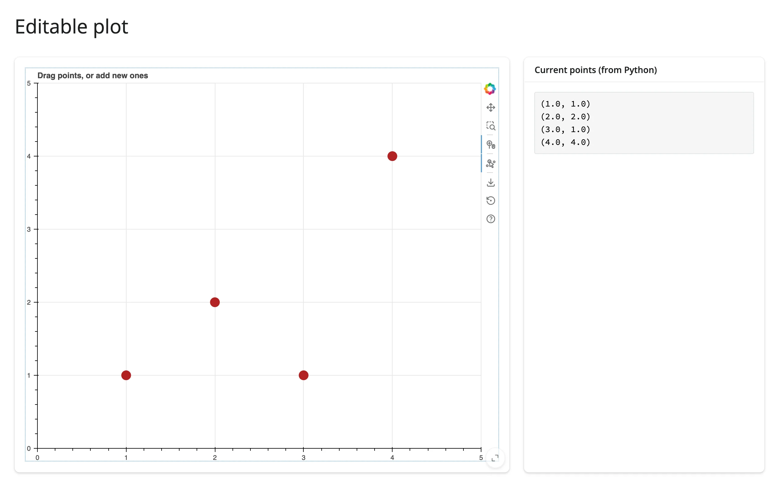
PointDrawTool (and Bokeh’s other edit tools) let a plot act as a data-entry form: users drag or add points, and Python receives the edited source.data through a plain on_change callback – the same bridge you’d use for anything the accessors don’t cover (see Beyond the accessors below):

examples/04_draw_tool.py35 lines

from bokeh.models import ColumnDataSource, PointDrawTool
from bokeh.plotting import figure
from shiny import reactive
from shiny.express import render, ui
from shinywidgets import render_bokeh

ui.page_opts(title="Editable plot", fillable=True)

edits = reactive.value(0)
src = ColumnDataSource({"x": [1, 2, 3], "y": [1, 2, 1]})
src.on_change("data", lambda attr, old, new: edits.set(edits() + 1))

with ui.layout_columns(col_widths=[8, 4]):
    with ui.card(full_screen=True):

        @render_bokeh
        def plot():
            p = figure(
                x_range=(0, 5), y_range=(0, 5), title="Drag points, or add new ones"
            )
            renderer = p.scatter("x", "y", source=src, size=15, color="firebrick")
            draw_tool = PointDrawTool(renderers=[renderer], add=True)
            p.add_tools(draw_tool)
            p.toolbar.active_tap = draw_tool
            return p

    with ui.card():
        ui.card_header("Current points (from Python)")

        @render.code
        def points():
            edits()  # re-run whenever the source's data changes
            return "\n".join(
                f"({x:.1f}, {y:.1f})" for x, y in zip(src.data["x"], src.data["y"])
            )

draw tool before draw tool after

Themes

Build a Document with a built-in theme, add your layout as its root, and return the layout (not the document):

examples/05_theme.py20 lines

import numpy as np
from bokeh.document import Document
from bokeh.plotting import figure
from bokeh.themes import built_in_themes
from shiny.express import ui
from shinywidgets import render_bokeh

ui.page_opts(title="A themed plot", fillable=True)

rng = np.random.default_rng(2)

with ui.card(full_screen=True):

    @render_bokeh
    def plot():
        doc = Document(theme=built_in_themes["night_sky"])
        p = figure(title="night_sky theme", sizing_mode="stretch_both")
        p.scatter(rng.normal(size=150), rng.normal(size=150), size=8, alpha=0.8)
        doc.add_root(p)
        return p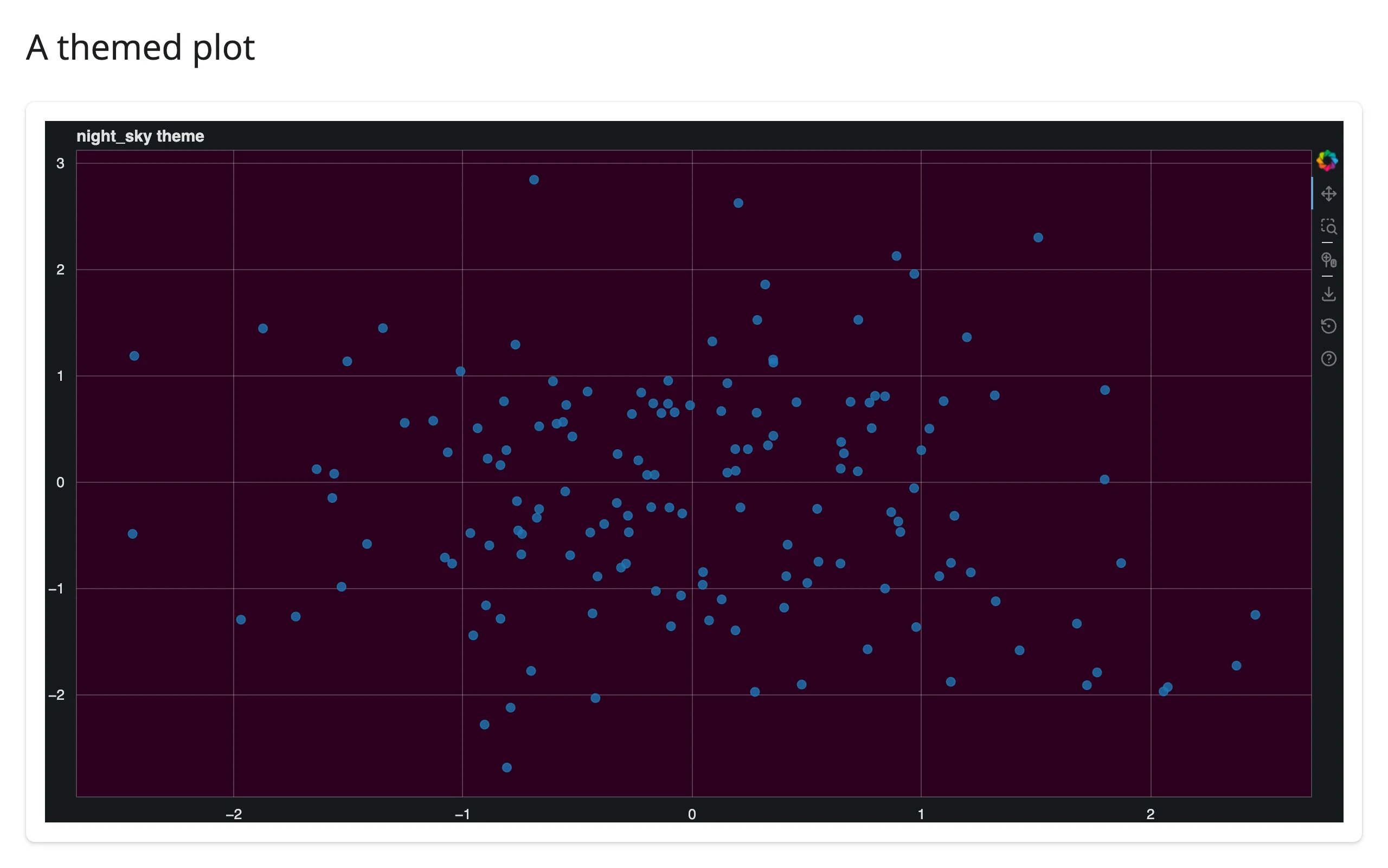

Client-only interactivity

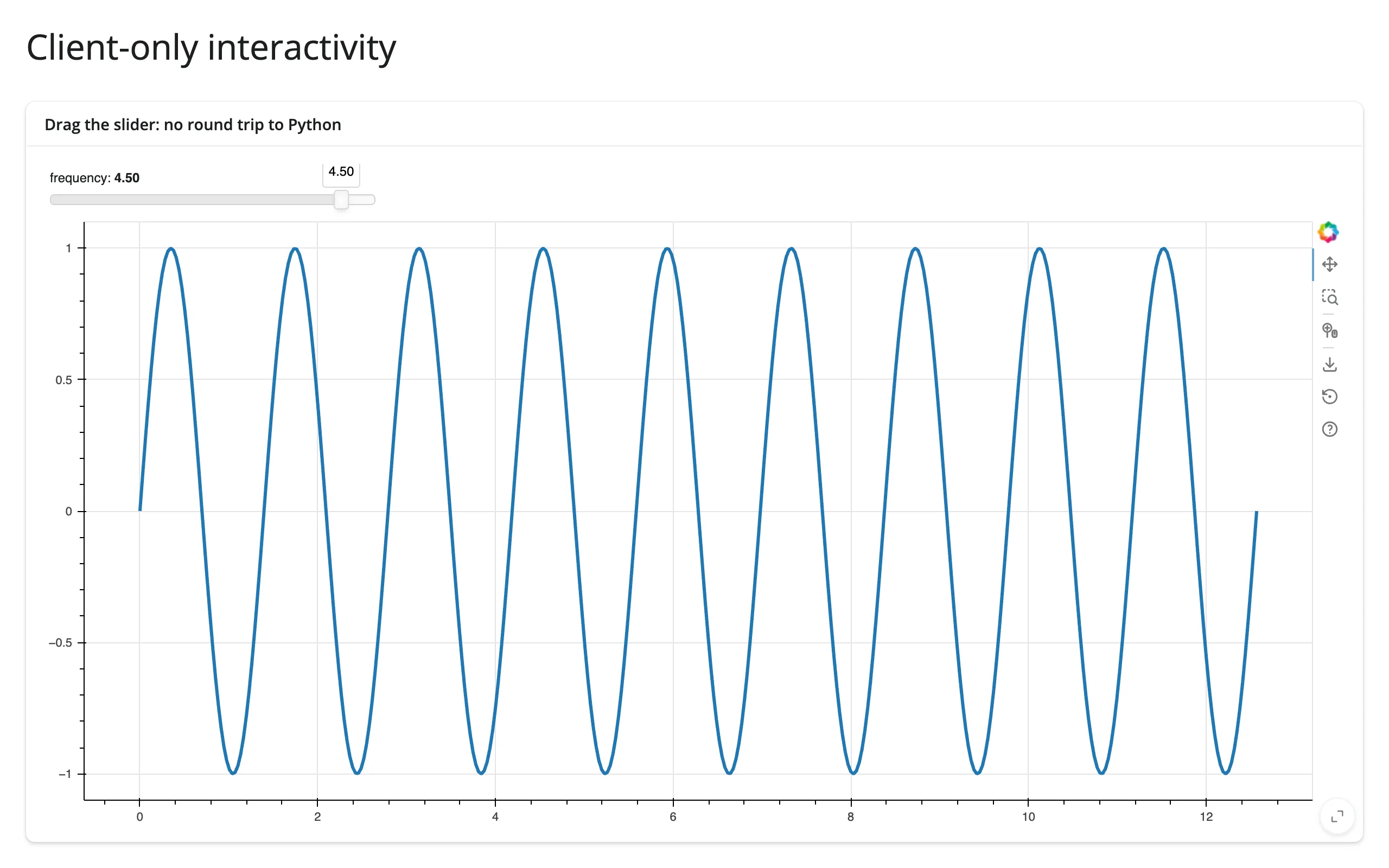
js_link() and CustomJS work exactly as they do in standalone Bokeh – useful for interactions that don’t need Python at all, like this frequency slider that rewrites a line’s data with no server round trip:

examples/06_js_link.py36 lines

import numpy as np
from bokeh.layouts import column
from bokeh.models import CustomJS, Slider
from bokeh.plotting import figure
from shiny.express import ui
from shinywidgets import render_bokeh

ui.page_opts(title="Client-only interactivity", fillable=True)

x = np.linspace(0, 4 * np.pi, 400)

with ui.card(full_screen=True):
    ui.card_header("Drag the slider: no round trip to Python")

    @render_bokeh
    def plot():
        p = figure(sizing_mode="stretch_both")
        line = p.line(x, np.sin(x), line_width=3)

        slider = Slider(start=0.1, end=5, value=1, step=0.1, title="frequency")
        slider.js_on_change(
            "value",
            CustomJS(
                args=dict(source=line.data_source, freq=slider),
                code="""
                const data = source.data
                const x = data['x']
                const y = data['y']
                for (let i = 0; i < x.length; i++) {
                    y[i] = Math.sin(freq.value * x[i])
                }
                source.change.emit()
                """,
            ),
        )
        return column(slider, p, sizing_mode="stretch_both")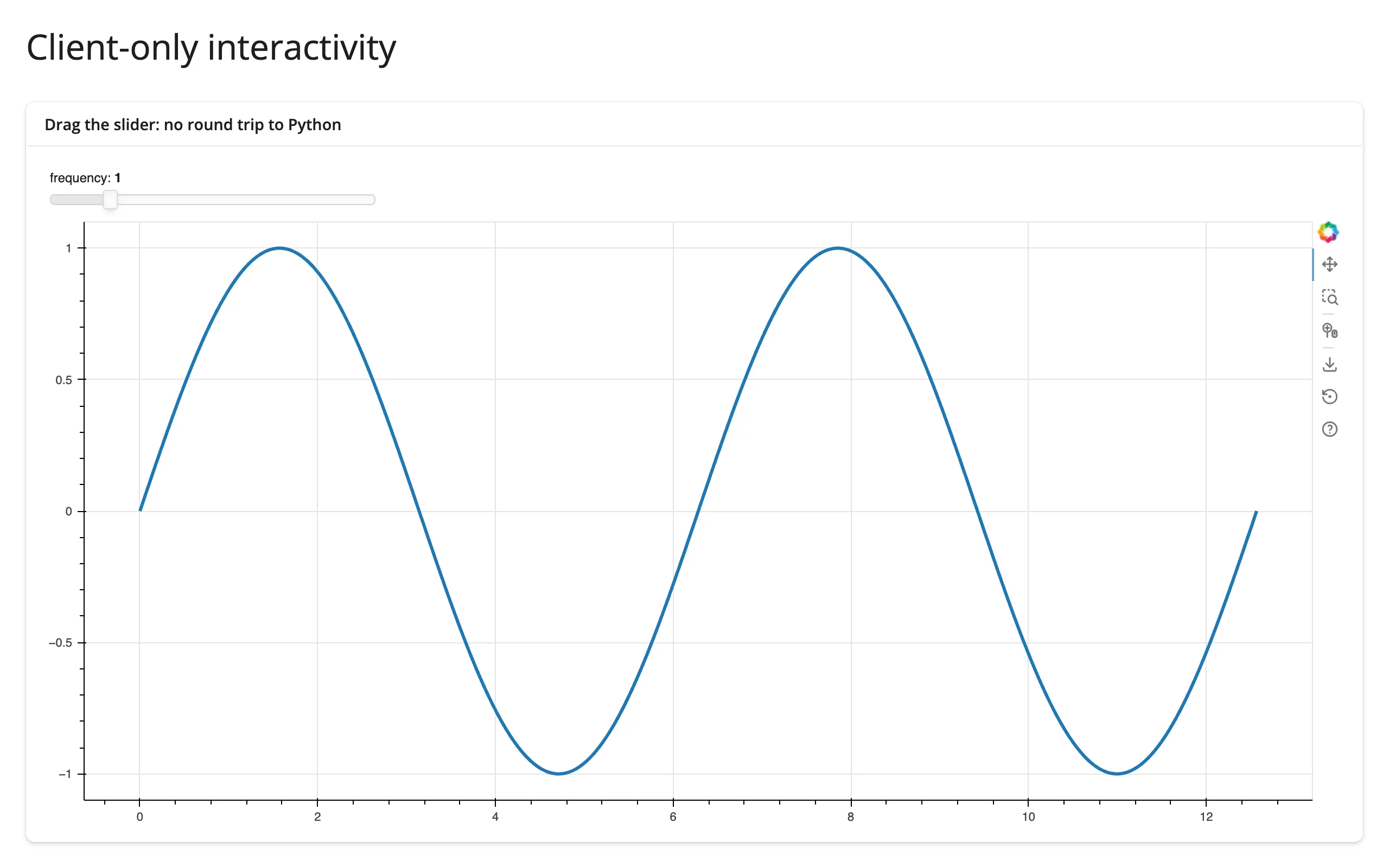

js_link before js_link after

Reacting to user interaction

Accessor reference

accessor	returns	before any interaction	across re-render	default rate policy
`selected()`	`list[int]`: row indices into the plot’s `ColumnDataSource`	`[]`	re-seeded from the new plot’s current selection (`[]` for a fresh plot)	debounce, 250 ms
`selected_rows()`	`pandas.DataFrame`: `source.to_df().iloc[indices]`	empty frame	follows `selected()`	follows `selected()`; the `source.data` part isn’t rate-limited
`tapped()`	`bokeh.events.Tap` (`.x`, `.y` in data units, `.model`)	`None`	kept – holds the previous plot’s last tap until the new plot is tapped	none – every tap re-runs readers
`zoomed()`	`bokeh.events.RangesUpdate` (`.x0`, `.x1`, `.y0`, `.y1`, `.model`)	seeded from the plot’s default ranges when they hold real values, else `None`	re-seeded from the new plot’s default ranges	none

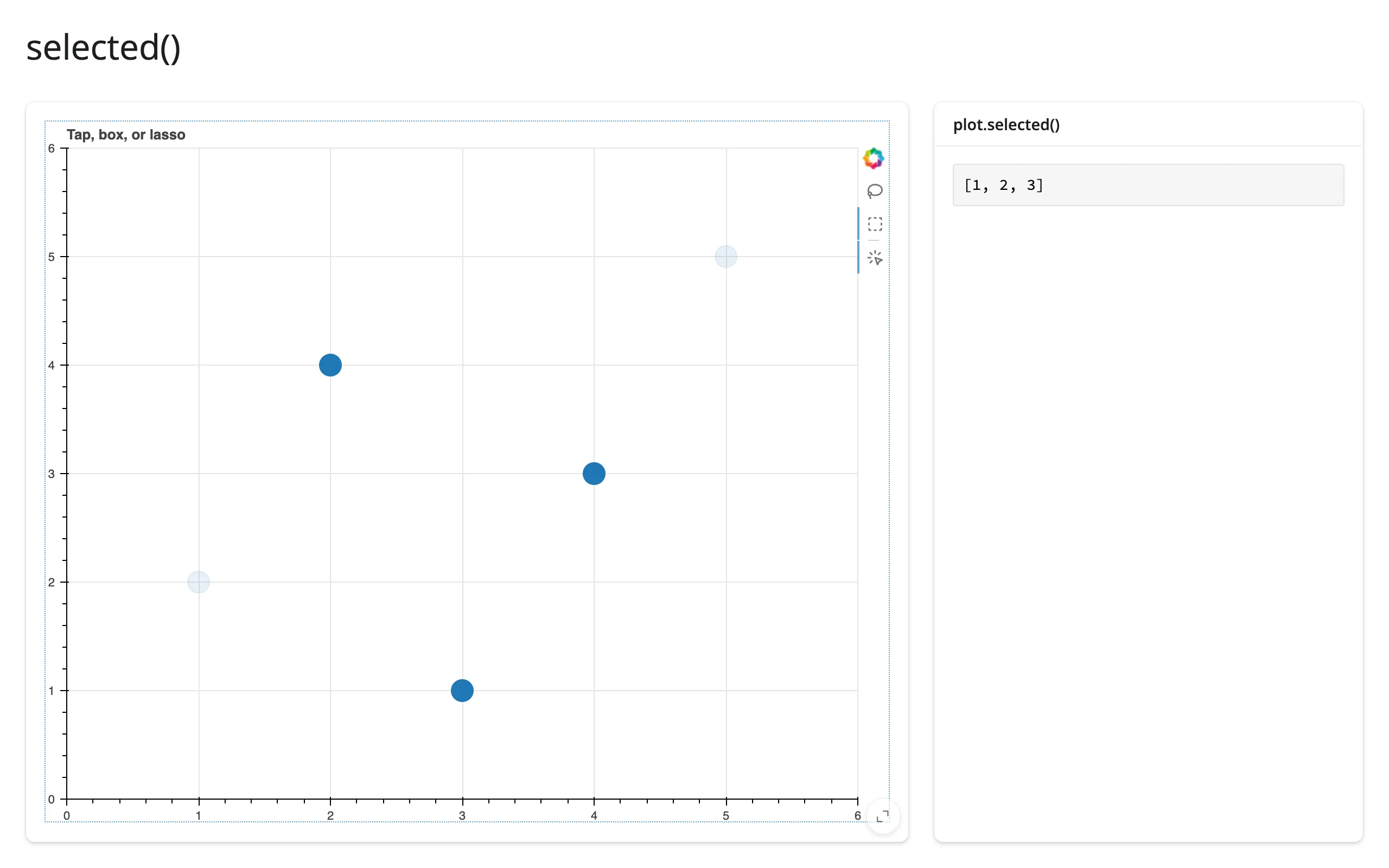
selected() and selected_rows() need a plot (or layout) with exactly one ColumnDataSource; with more than one, they raise a TypeError that points you at source.selected.on_change("indices", ...) instead (see Several ColumnDataSources below). A re-render gives the user a brand new plot, but no accessor needs a warm-up read to start tracking it: all four attach the moment the plot renders, whether or not anything has read them yet. What happens to their value on a re-render differs by what they track: tapped() is a record of something the user did, so it’s kept until they tap the new plot; selected() and zoomed() describe the plot’s own current state, so they re-seed from the new plot (an unselected plot’s selected() is []; a plot whose ranges have real default values seeds zoomed() with them). None of the four can be read inside the same @render_bokeh function that builds the plot – doing so raises a RuntimeError pointing you at a @reactive.effect instead, since the render function doesn’t have a widget to read from yet.

`selected()`

examples/07_selected.py32 lines

from bokeh.models import ColumnDataSource
from bokeh.plotting import figure
from shiny.express import render, ui
from shinywidgets import render_bokeh

ui.page_opts(title="selected()", fillable=True)

src = ColumnDataSource(
    {"x": [1, 2, 3, 4, 5], "y": [2, 4, 1, 3, 5], "name": list("abcde")}
)

with ui.layout_columns(col_widths=[8, 4]):
    with ui.card(full_screen=True):

        @render_bokeh
        def plot():
            p = figure(
                x_range=(0, 6),
                y_range=(0, 6),
                tools="tap,box_select,lasso_select",
                active_drag="box_select",
                title="Tap, box, or lasso",
            )
            p.scatter("x", "y", source=src, size=20)
            return p

    with ui.card():
        ui.card_header("plot.selected()")

        @render.code
        def selected():
            return str(plot.selected())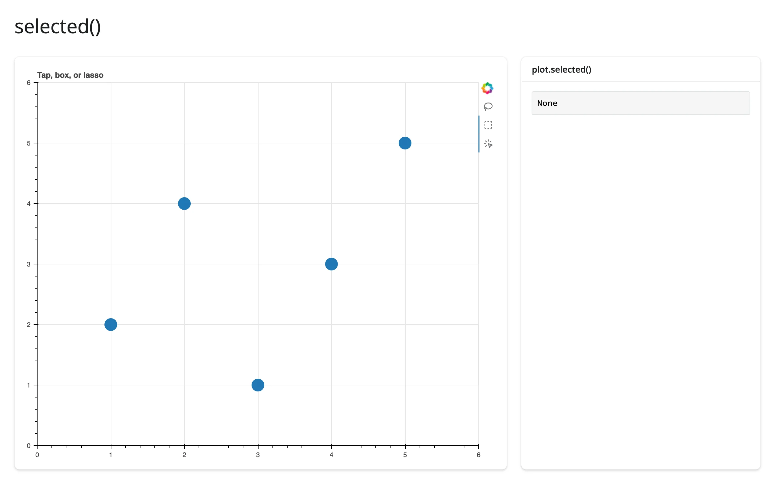

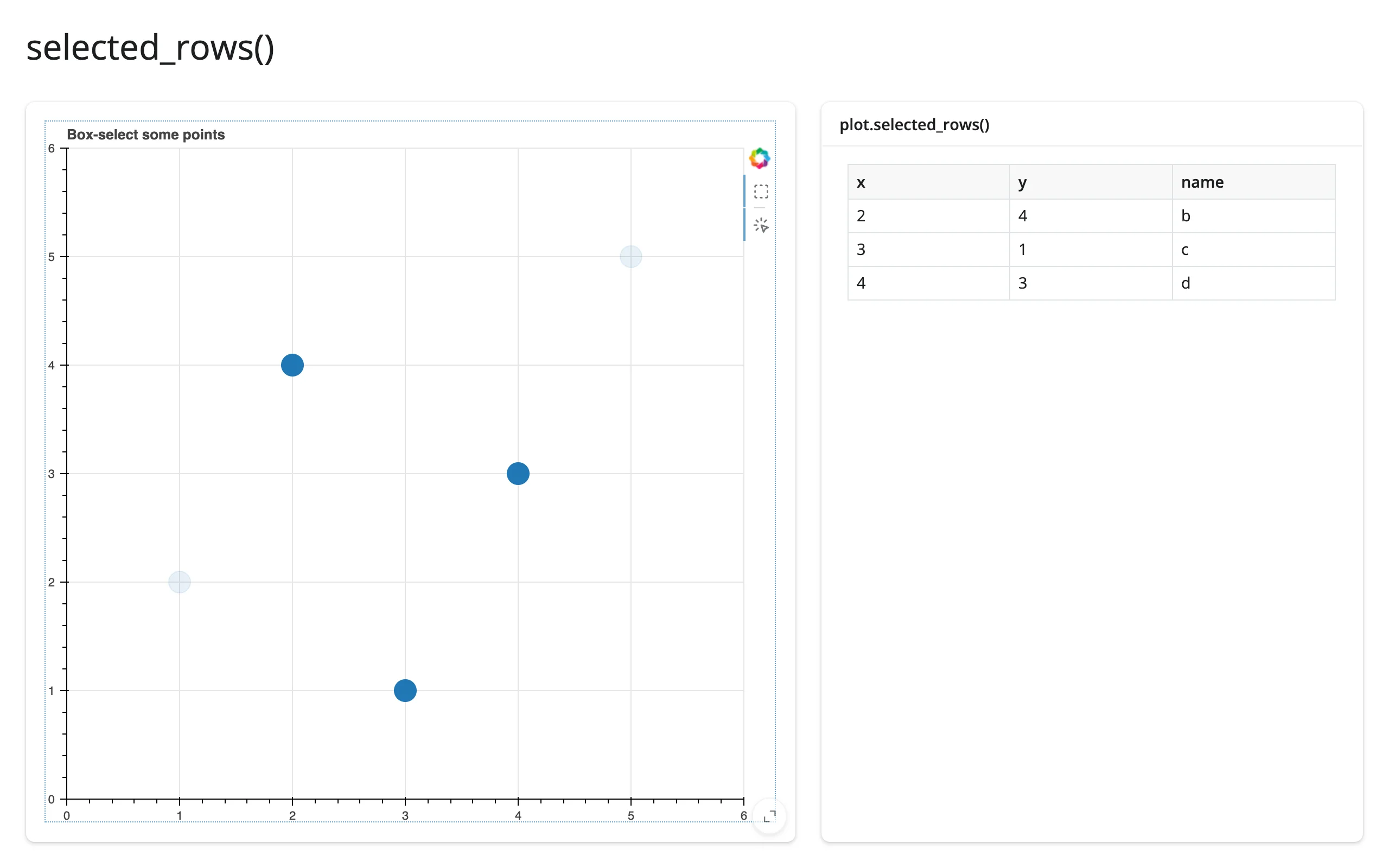
selected before selected after

`selected_rows()`

examples/08_selected_rows.py36 lines

from bokeh.models import ColumnDataSource
from bokeh.plotting import figure
from shiny.express import render, ui
from shinywidgets import render_bokeh

ui.page_opts(title="selected_rows()", fillable=True)

src = ColumnDataSource(
    {
        "x": [1, 2, 3, 4, 5],
        "y": [2, 4, 1, 3, 5],
        "name": list("abcde"),
    }
)

with ui.layout_columns(col_widths=[7, 5]):
    with ui.card(full_screen=True):

        @render_bokeh
        def plot():
            p = figure(
                x_range=(0, 6),
                y_range=(0, 6),
                tools="tap,box_select",
                active_drag="box_select",
                title="Box-select some points",
            )
            p.scatter("x", "y", source=src, size=20)
            return p

    with ui.card():
        ui.card_header("plot.selected_rows()")

        @render.data_frame
        def rows():
            return plot.selected_rows()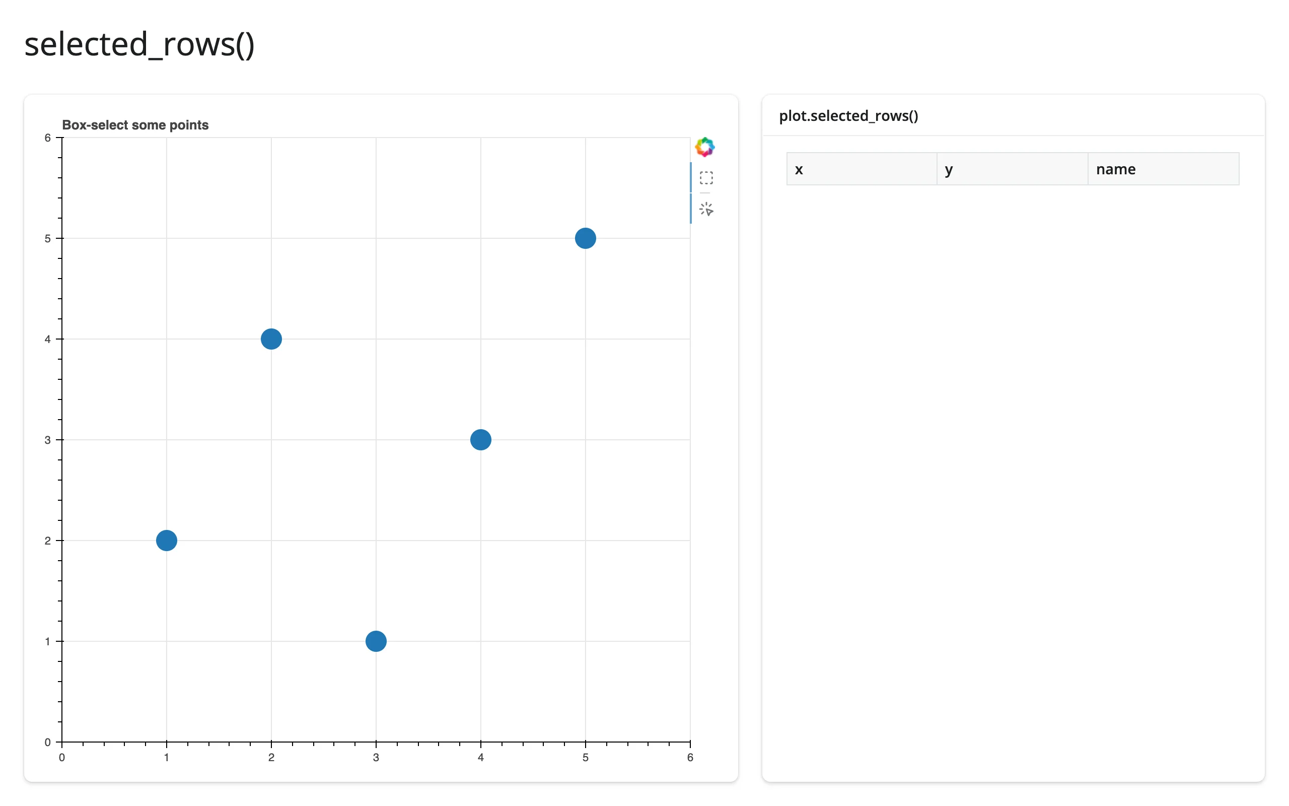

selected_rows before selected_rows after

`tapped()`

examples/09_tapped.py23 lines

from bokeh.plotting import figure
from shiny import req
from shiny.express import render, ui
from shinywidgets import render_bokeh

ui.page_opts(title="tapped()", fillable=True)

with ui.layout_columns(col_widths=[8, 4]):
    with ui.card(full_screen=True):

        @render_bokeh
        def plot():
            p = figure(x_range=(0, 10), y_range=(0, 10), tools="tap", title="Click anywhere")
            p.scatter([2, 5, 8], [2, 5, 8], size=20)
            return p

    with ui.card():
        ui.card_header("plot.tapped()")

        @render.text
        def coords():
            t = req(plot.tapped())
            return f"({t.x:.2f}, {t.y:.2f})"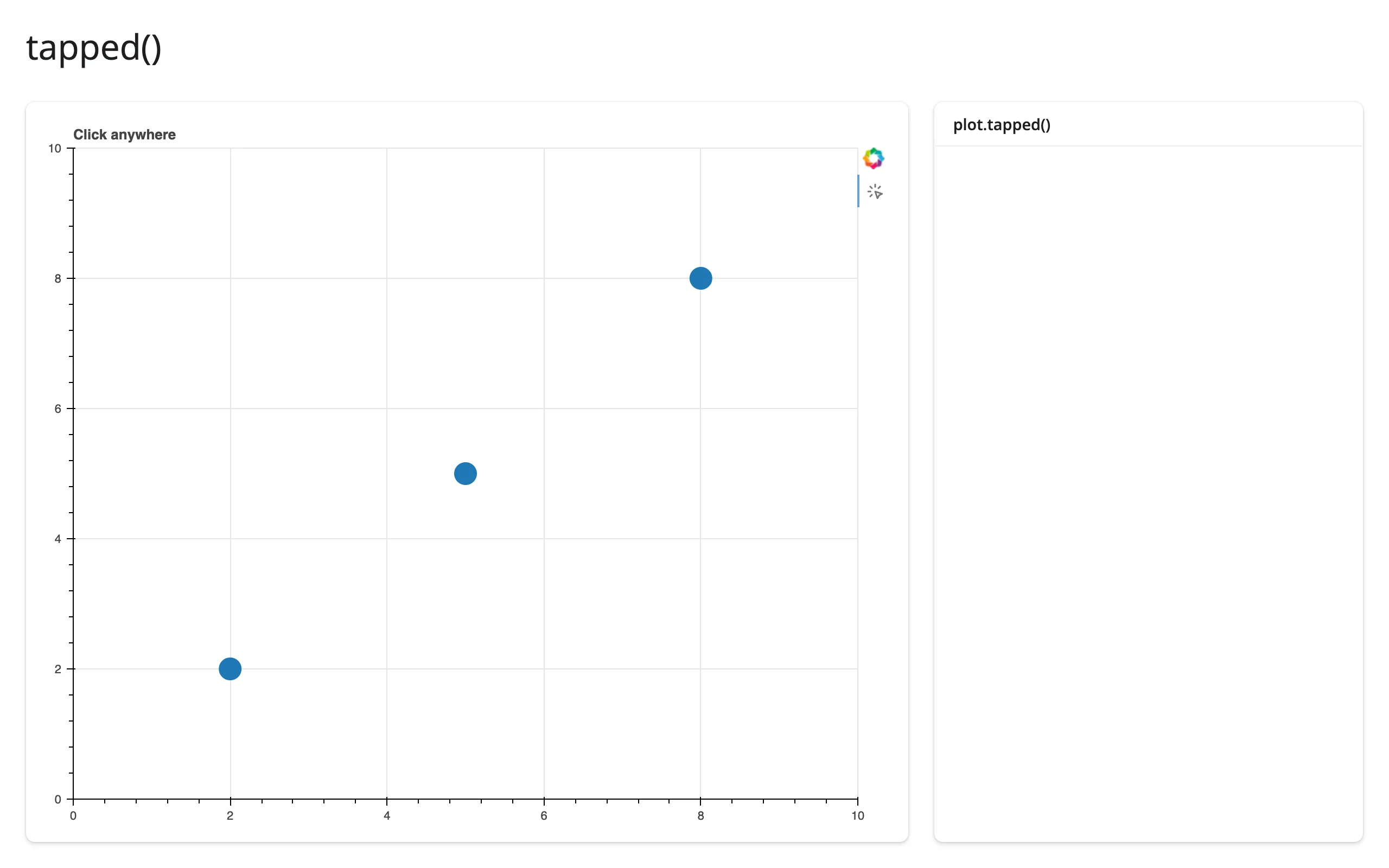

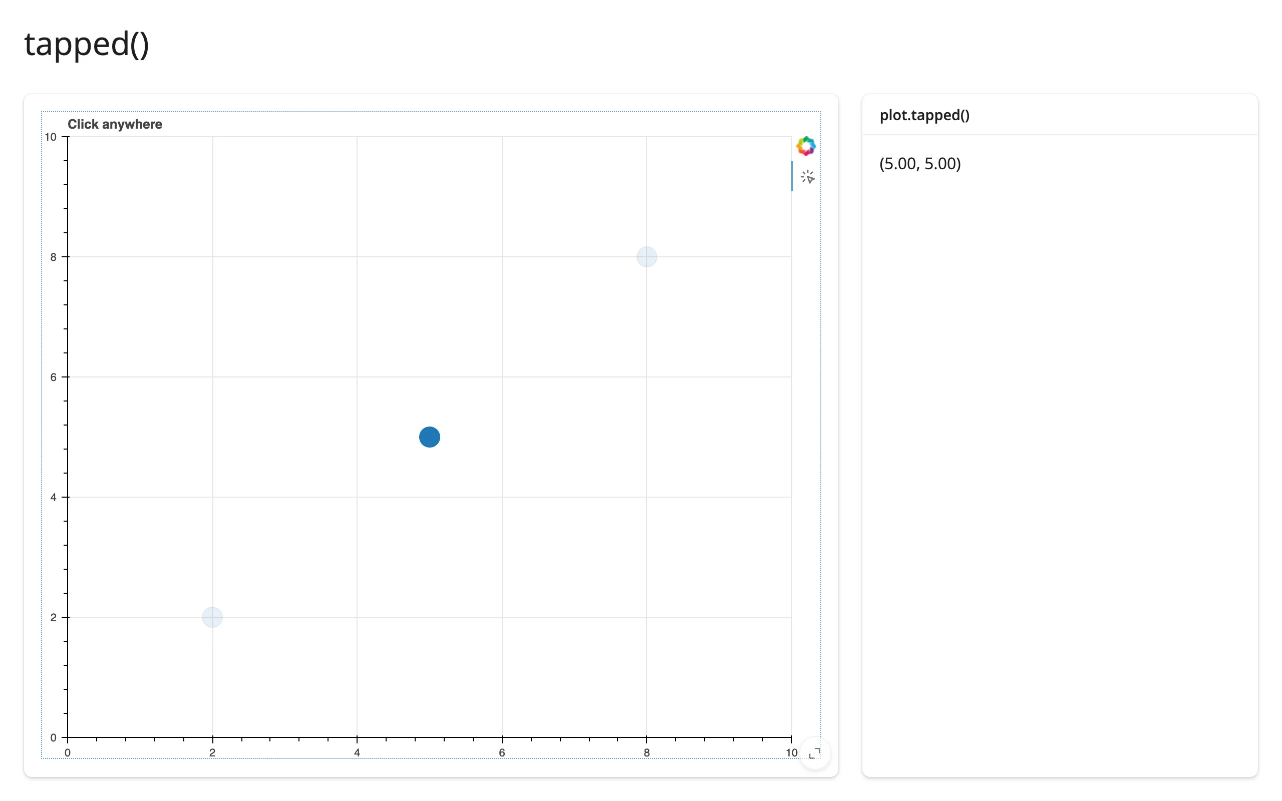
tapped before tapped after

`zoomed()`

examples/10_zoomed.py31 lines

import numpy as np
from bokeh.plotting import figure
from shiny import req
from shiny.express import render, ui
from shinywidgets import render_bokeh

ui.page_opts(title="zoomed()", fillable=True)

rng = np.random.default_rng(3)
x = rng.normal(size=300)
y = rng.normal(size=300)

with ui.layout_columns(col_widths=[8, 4]):
    with ui.card(full_screen=True):

        @render_bokeh
        def plot():
            p = figure(tools="pan,wheel_zoom,reset", active_scroll="wheel_zoom")
            p.scatter(x, y, size=6, alpha=0.6)
            return p

    with ui.card():
        ui.card_header("plot.zoomed()")

        @render.text
        def ranges():
            z = req(plot.zoomed())
            return (
                f"x: [{z.x0:.2f}, {z.x1:.2f}]\n"
                f"y: [{z.y0:.2f}, {z.y1:.2f}]"
            )

zoomed before zoomed after

Several ColumnDataSources

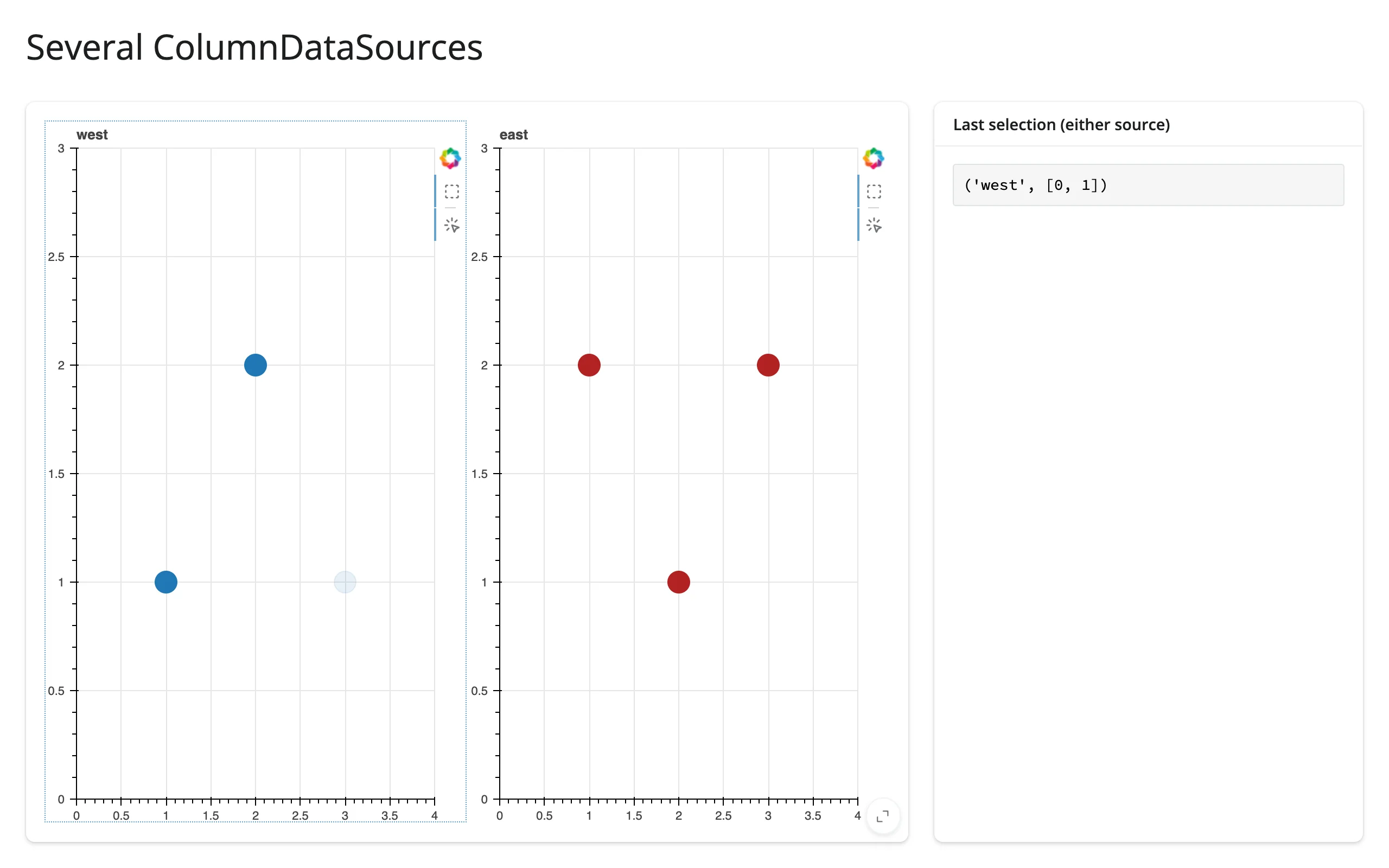
A dashboard with two unrelated plots in one @render_bokeh output can’t use selected() – it would be ambiguous which source’s selection you meant. Wire each source’s own on_change into a reactive.value instead; it’s the same mechanism the accessors use internally, just addressed to a specific source:

examples/11_multiple_sources.py49 lines

from bokeh.layouts import row
from bokeh.models import ColumnDataSource
from bokeh.plotting import figure
from shiny import reactive
from shiny.express import render, ui
from shinywidgets import render_bokeh

ui.page_opts(title="Several ColumnDataSources", fillable=True)

west = ColumnDataSource({"x": [1, 2, 3], "y": [1, 2, 1], "name": list("abc")})
east = ColumnDataSource({"x": [1, 2, 3], "y": [2, 1, 2], "name": list("def")})

# plot.selected() would raise TypeError here (two sources). Wire each
# source's own callback into a reactive.value instead.
picked = reactive.value(None)
west.selected.on_change("indices", lambda attr, old, new: picked.set(("west", new)))
east.selected.on_change("indices", lambda attr, old, new: picked.set(("east", new)))

with ui.layout_columns(col_widths=[8, 4]):
    with ui.card(full_screen=True):

        @render_bokeh
        def plot():
            left = figure(
                title="west",
                tools="tap,box_select",
                active_drag="box_select",
                x_range=(0, 4),
                y_range=(0, 3),
                sizing_mode="stretch_both",
            )
            left.scatter("x", "y", source=west, size=20)
            right = figure(
                title="east",
                tools="tap,box_select",
                active_drag="box_select",
                x_range=(0, 4),
                y_range=(0, 3),
                sizing_mode="stretch_both",
            )
            right.scatter("x", "y", source=east, size=20, color="firebrick")
            return row(left, right, sizing_mode="stretch_both")

    with ui.card():
        ui.card_header("Last selection (either source)")

        @render.code
        def selection():
            return str(picked())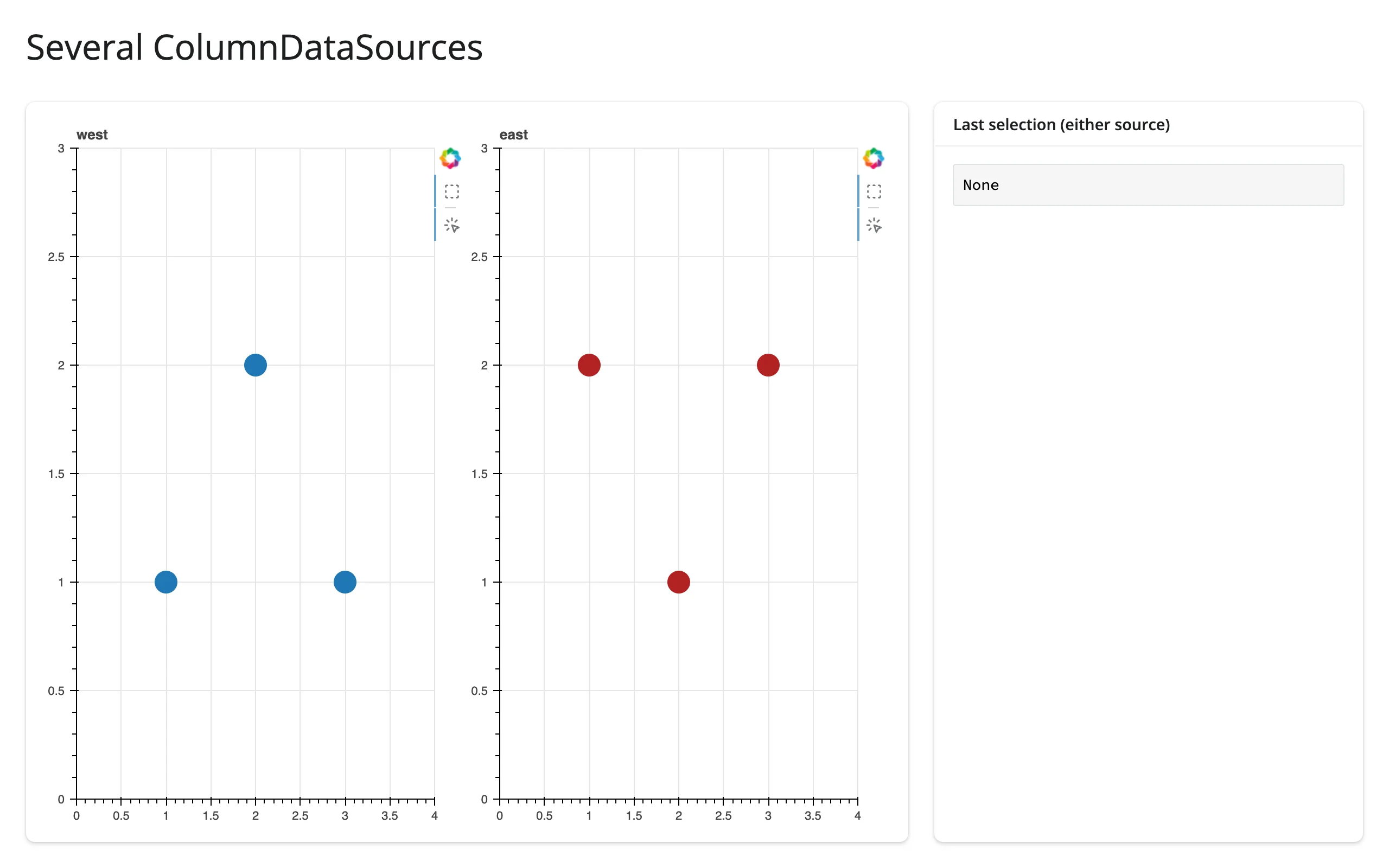

multiple sources before multiple sources after

Beyond the accessors: `reactive_read`

BokehModel (the ipywidget @render_bokeh builds) has no useful synced traits – checked directly against jupyter_bokeh on the current version: its only public traits are combine_events, comm, keys, layout, log, render_bundle, tabbable, and tooltip, none of which reflect selection, ranges, or anything else happening in the plot. So reactive_read(plot.widget, ...) has nothing to offer here, unlike widgets whose state genuinely lives in ipywidget traits. Everything Bokeh reports arrives instead as ordinary Python-side changes to the Bokeh objects themselves (source.selected.indices, range.start, a Slider’s value, …), which is what the four accessors read and what the raw on_change()/on_event() bridge in the examples above reaches for everything else – Bokeh widgets, draw-tool edits, and multiple sources.

Rate limiting

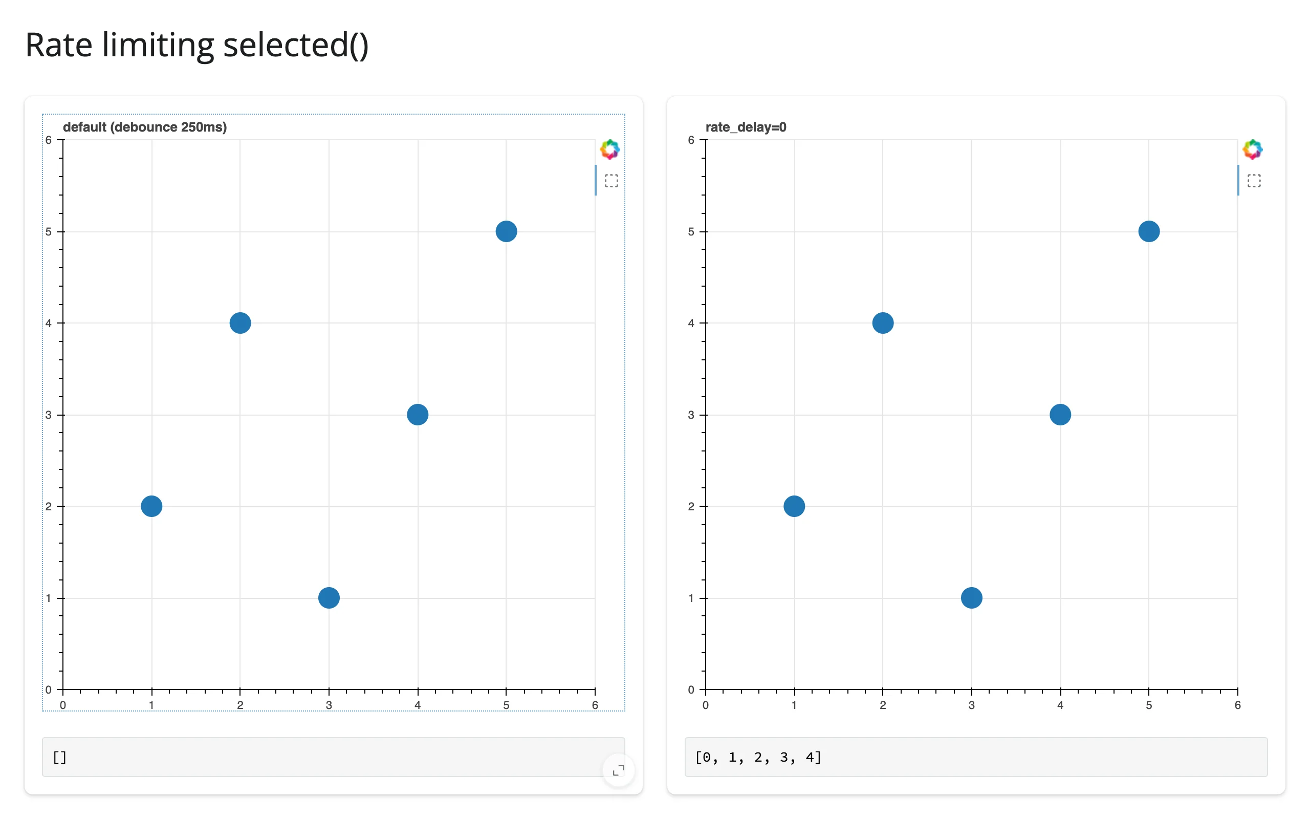
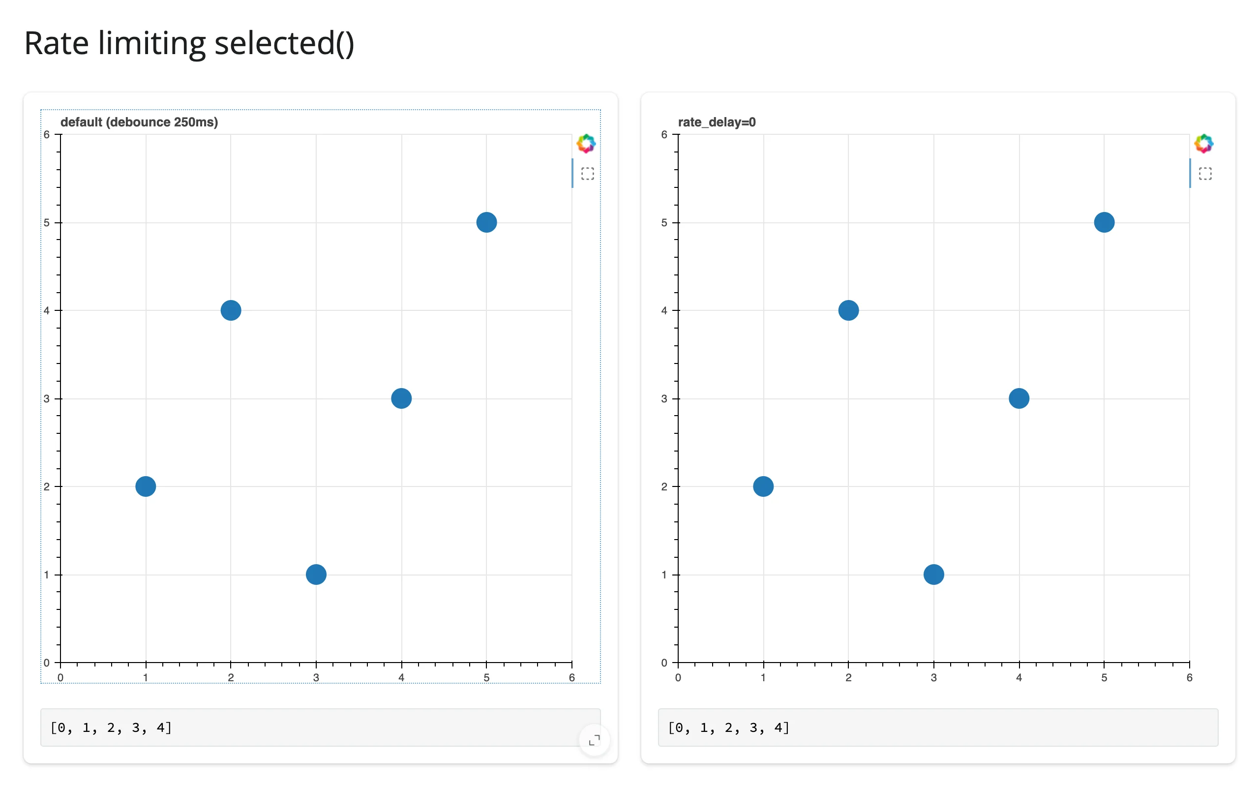
selected() debounces by default (rate_policy="debounce", rate_delay=0.25), so a slow lasso only reports its final shape. Pass rate_delay=0 to @render_bokeh to see every intermediate selection as the user drags – useful for a live preview, at the cost of more reactive re-runs. tapped() and zoomed() aren’t rate-limited at all (Bokeh already reports once per gesture), so there’s nothing to tune for them.

examples/12_rate_limiting.py44 lines

from bokeh.models import ColumnDataSource
from bokeh.plotting import figure
from shiny.express import render, ui
from shinywidgets import render_bokeh

ui.page_opts(title="Rate limiting selected()", fillable=True)


def points():
    return ColumnDataSource({"x": [1, 2, 3, 4, 5], "y": [2, 4, 1, 3, 5]})


def scatter(title):
    p = figure(
        x_range=(0, 6),
        y_range=(0, 6),
        tools="box_select",
        active_drag="box_select",
        title=title,
    )
    p.scatter("x", "y", source=points(), size=20)
    return p


with ui.layout_columns():
    with ui.card(full_screen=True):

        @render_bokeh  # default: debounced 250ms
        def default_plot():
            return scatter("default (debounce 250ms)")

        @render.code
        def default_selected():
            return str(default_plot.selected())

    with ui.card(full_screen=True):

        @render_bokeh(rate_delay=0)  # report every change immediately
        def instant_plot():
            return scatter("rate_delay=0")

        @render.code
        def instant_selected():
            return str(instant_plot.selected())

The same box-select gesture, same instant (no-wait) screenshot: the default plot hasn’t caught up yet (still [], its seeded empty value), the rate_delay=0 plot already has:

rate limiting default, no wait rate limiting instant, no wait

Reading an accessor on demand

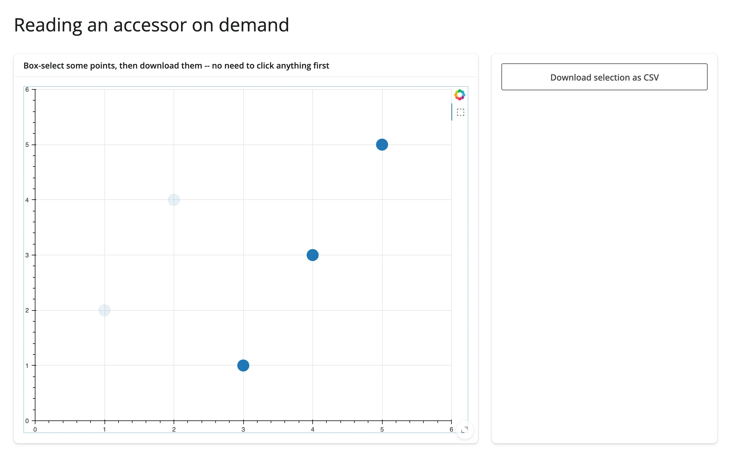
Every accessor is live the moment its plot renders – it doesn’t need a prior read to start tracking interactions. That makes it safe to read one somewhere that only runs occasionally, like a download handler: the value it gets back is whatever the user last did, even on the handler’s very first run.

examples/17_download_selection.py36 lines

from bokeh.models import ColumnDataSource
from bokeh.plotting import figure
from shiny.express import render, ui
from shinywidgets import render_bokeh

ui.page_opts(title="Reading an accessor on demand", fillable=True)

src = ColumnDataSource(
    {"x": [1, 2, 3, 4, 5], "y": [2, 4, 1, 3, 5], "name": list("abcde")}
)

with ui.layout_columns(col_widths=[8, 4]):
    with ui.card(full_screen=True):
        ui.card_header("Box-select some points, then download them -- no need to click anything first")

        @render_bokeh
        def plot():
            p = figure(
                x_range=(0, 6),
                y_range=(0, 6),
                tools="box_select",
                active_drag="box_select",
            )
            p.scatter("x", "y", source=src, size=20)
            return p

    with ui.card():

        @render.download_button(
            filename="selection.csv", label="Download selection as CSV"
        )
        def download():
            # plot.selected_rows() is live the moment the plot renders, so
            # this reads whatever is currently selected -- even if the
            # download handler itself has never run before.
            yield plot.selected_rows().to_csv(index=False)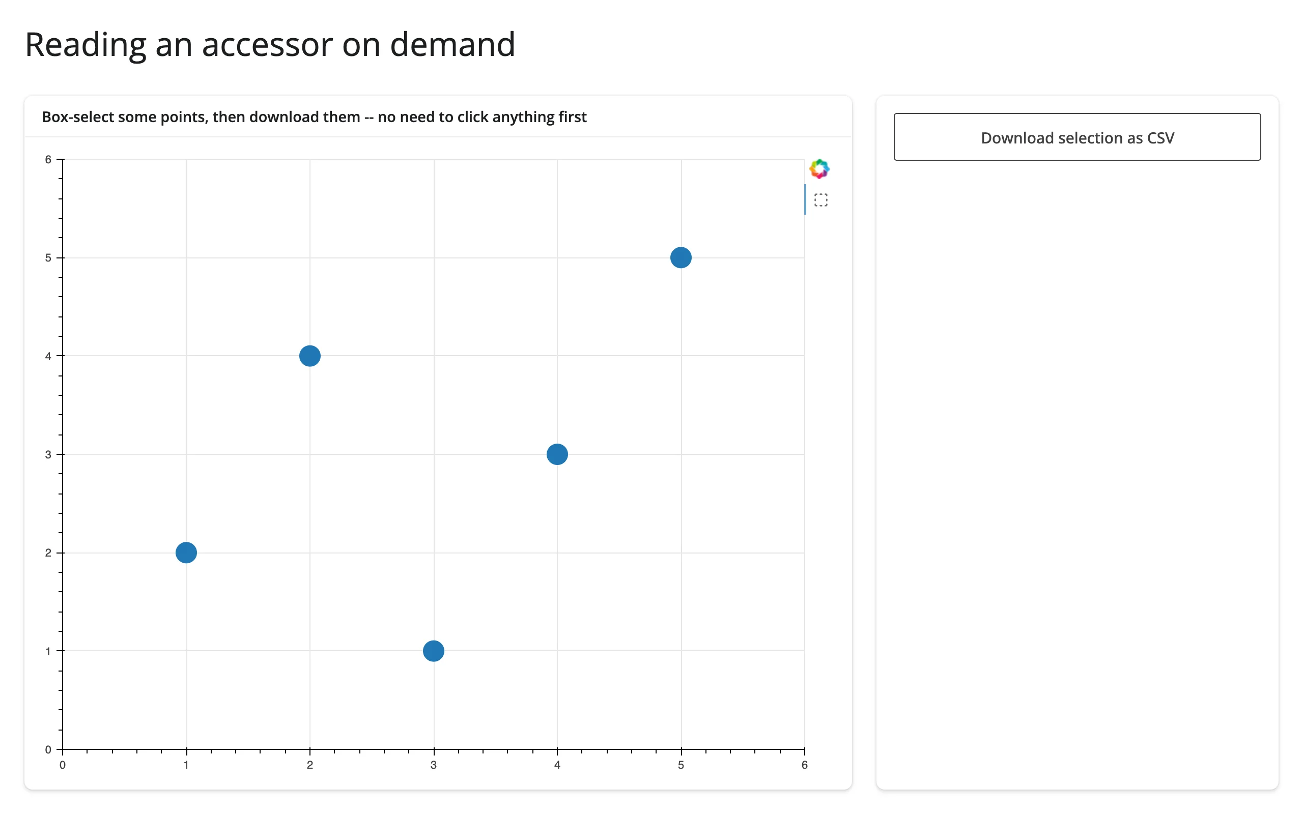

download selection before download selection after

Updating the widget from Python

Because a Bokeh plot is a tree of live objects, you rarely need to rebuild it to change what it shows. Keep a Python reference to the pieces you’ll change (a module- or session-level ColumnDataSource, as in the examples above), and mutate them from a @reactive.effect that runs independently of the render function. This matters because re-rendering gives the user a brand new plot – their zoom, pan, and selection all go back to the plot’s defaults, and selected()/zoomed() re-seed from those defaults too (see the accessor reference above) – while an in-place update leaves all of it alone and sends a small patch instead of the whole document again:

examples/13_update_in_place.py29 lines

import numpy as np
from bokeh.models import ColumnDataSource
from bokeh.plotting import figure
from shiny import reactive
from shiny.express import input, render, ui
from shinywidgets import render_bokeh

ui.page_opts(title="Update in place", fillable=True)

rng = np.random.default_rng(4)
full_x, full_y = rng.normal(size=200), rng.normal(size=200)
src = ColumnDataSource({"x": full_x, "y": full_y})

with ui.card(full_screen=True):
    ui.input_slider("n", "Number of points", min=20, max=200, value=200, step=20)

    @render_bokeh
    def plot():
        p = figure(title="Pan or zoom, then move the slider")
        p.scatter("x", "y", source=src, size=6, alpha=0.6)
        return p


@reactive.effect
def _():
    # Mutates the existing ColumnDataSource instead of returning a new
    # figure, so the user's current zoom/pan survives the update.
    n = input.n()
    src.data = {"x": full_x[:n], "y": full_y[:n]}

Panned and zoomed (top-left), then the slider cut the point count to 100 – the view didn’t reset:

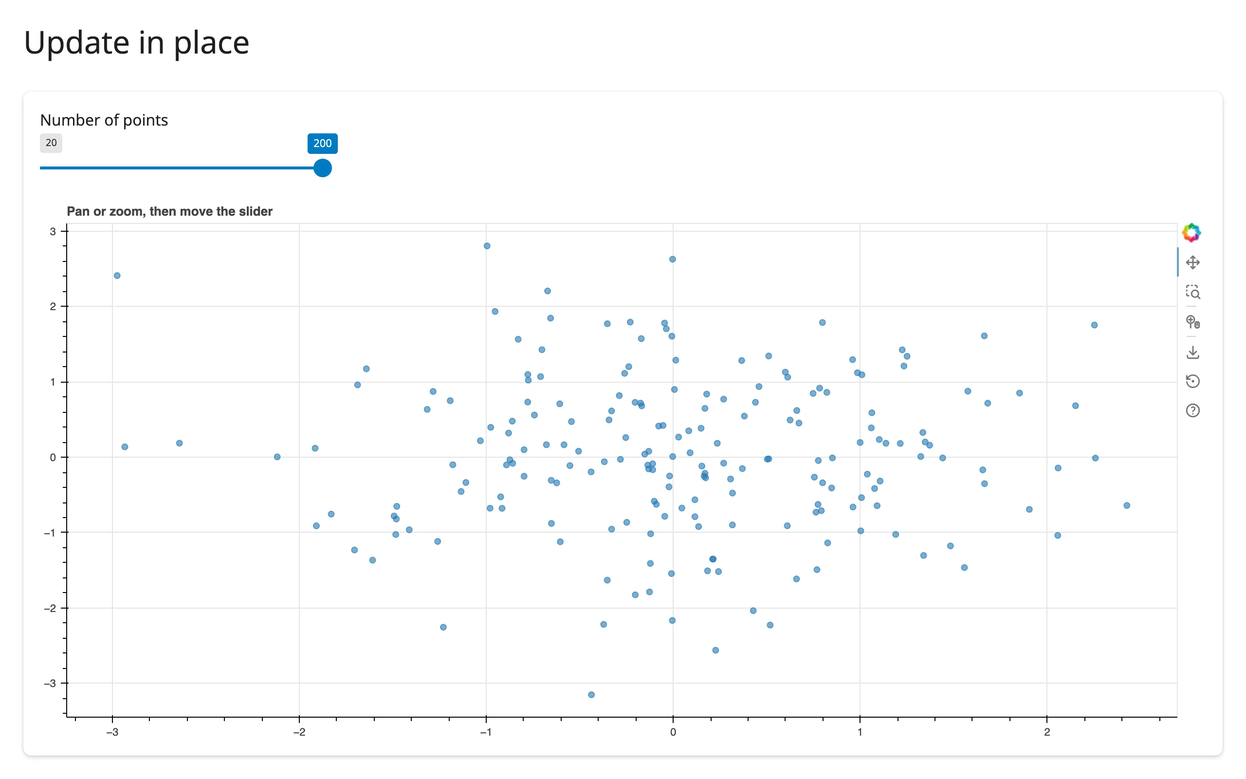
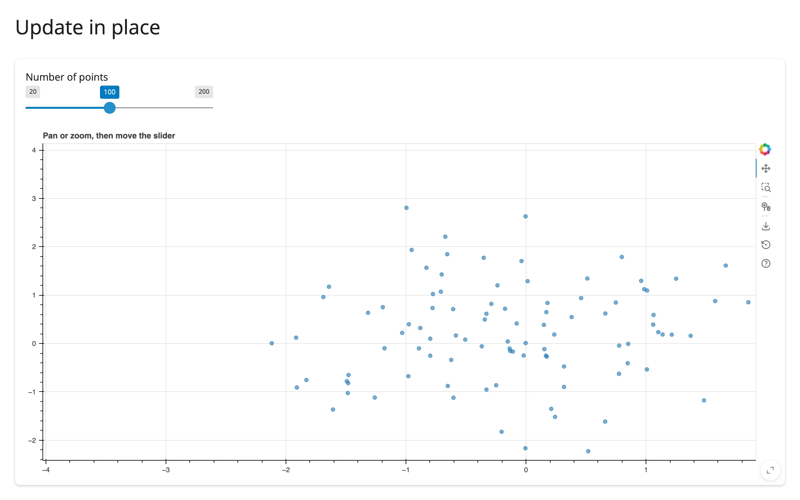
src.data = {...} replaces the whole source; src.data["col"] = arr patches a single column (used by the rate-limiting and periodic-table examples above to resize markers without touching anything else); src.patch() updates specific rows. If the effect needs to read an input that shouldn’t itself trigger the update, wrap just that read in with reactive.isolate(): ... – not needed here, since input.n() is the only input this effect cares about.

Coordinating multiple views

Linked brushing, with Python in the loop

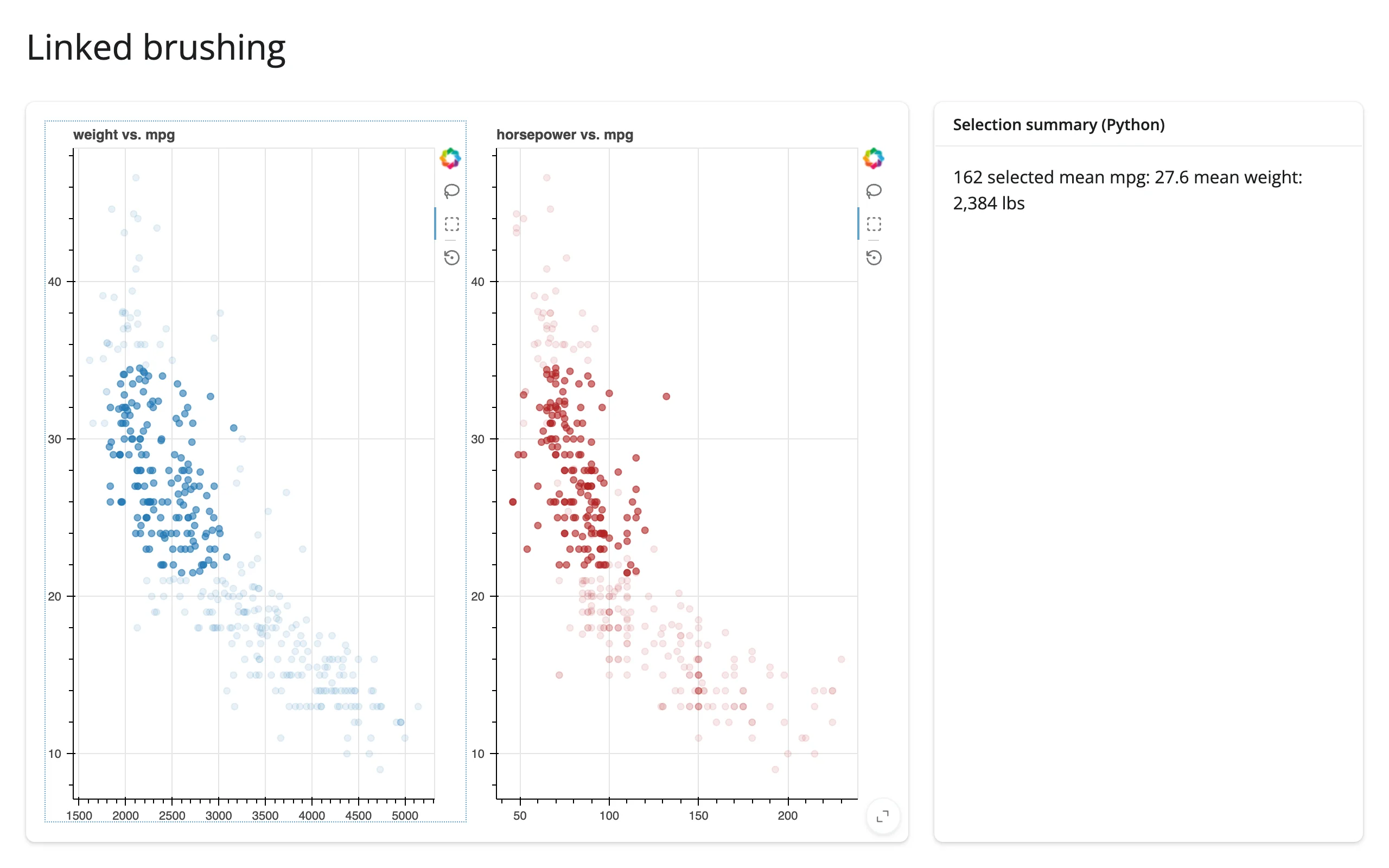
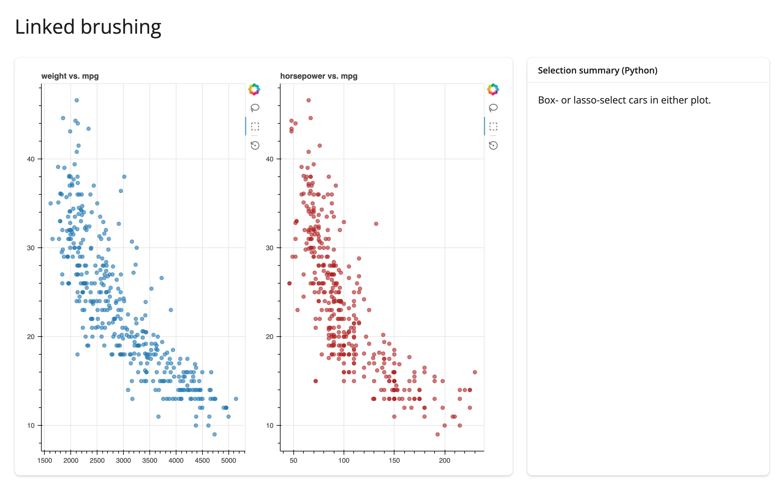
Give two figures the same ColumnDataSource and return them together from one @render_bokeh function (a source can belong to only one Bokeh document, so linked plots can’t come from separate outputs). The link itself is instant and entirely in the browser; Python still sees the selection through selected_rows(), so a sidebar can summarize it live:

examples/14_linked_brushing.py46 lines

# Uses bokeh's own sample-data package (downloaded on first use):
#   pip install bokeh_sampledata
from bokeh.layouts import row
from bokeh.models import ColumnDataSource
from bokeh.plotting import figure
from bokeh.sampledata.autompg import autompg
from shiny.express import render, ui
from shinywidgets import render_bokeh

ui.page_opts(title="Linked brushing", fillable=True)

src = ColumnDataSource(autompg)

with ui.layout_columns(col_widths=[8, 4]):
    with ui.card(full_screen=True):

        @render_bokeh
        def plots():
            tools = "box_select,lasso_select,reset"
            left = figure(
                title="weight vs. mpg", tools=tools, active_drag="box_select",
                sizing_mode="stretch_both",
            )
            left.scatter("weight", "mpg", source=src, size=6, alpha=0.6)

            right = figure(
                title="horsepower vs. mpg", tools=tools, active_drag="box_select",
                sizing_mode="stretch_both",
            )
            right.scatter("hp", "mpg", source=src, size=6, alpha=0.6, color="firebrick")

            return row(left, right, sizing_mode="stretch_both")

    with ui.card():
        ui.card_header("Selection summary (Python)")

        @render.text
        def summary():
            rows = plots.selected_rows()
            if len(rows) == 0:
                return "Box- or lasso-select cars in either plot."
            return (
                f"{len(rows)} selected\n"
                f"mean mpg: {rows['mpg'].mean():.1f}\n"
                f"mean weight: {rows['weight'].mean():,.0f} lbs"
            )

Box-selecting the lighter, more fuel-efficient cars in the left plot highlights the same 162 cars in the horsepower plot, and the sidebar’s mean mpg/weight update through selected_rows():

linked brushing before linked brushing after

A Bokeh selection driving a different widget entirely

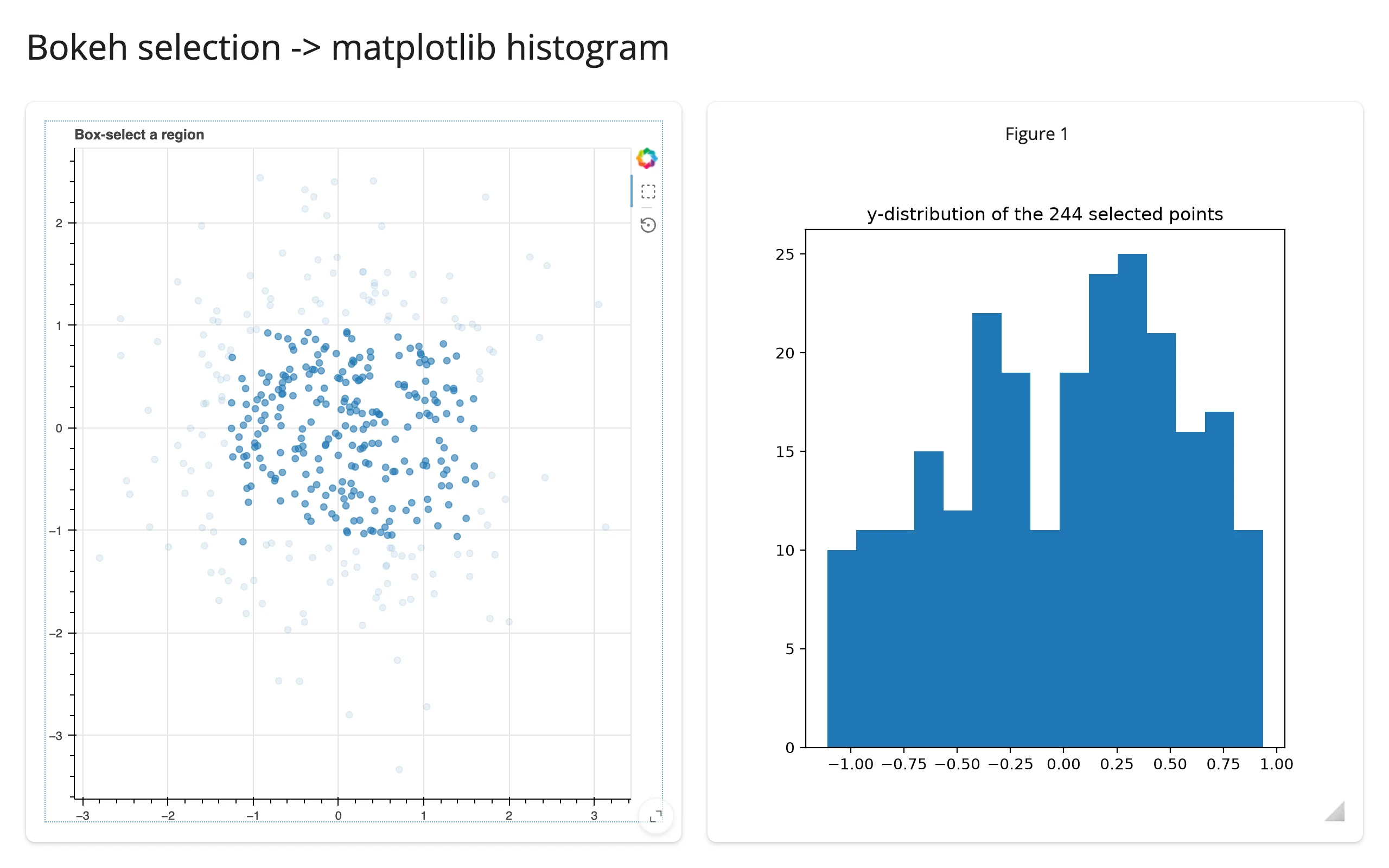
selected() is just a Python list once you have it, so nothing ties it to Bokeh on the receiving end. Here a box-select in a Bokeh scatter plot drives a live matplotlib histogram of the selected points – the same pattern works for render_reactable, render_itables, or any other output:

examples/15_lasso_to_histogram.py34 lines

import matplotlib.pyplot as plt
import numpy as np
from bokeh.models import ColumnDataSource
from bokeh.plotting import figure
from shiny.express import render, ui
from shinywidgets import render_bokeh, render_matplotlib

ui.page_opts(title="Bokeh selection -> matplotlib histogram", fillable=True)

rng = np.random.default_rng(6)
src = ColumnDataSource({"x": rng.normal(size=400), "y": rng.normal(size=400)})

with ui.layout_columns():
    with ui.card(full_screen=True):

        @render_bokeh
        def scatter():
            p = figure(
                title="Box-select a region",
                tools="box_select,reset",
                active_drag="box_select",
            )
            p.scatter("x", "y", source=src, size=6, alpha=0.6)
            return p

    with ui.card(full_screen=True):

        @render_matplotlib
        def hist():
            indices = scatter.selected() or []
            fig, ax = plt.subplots()
            ax.hist(np.asarray(src.data["y"])[indices], bins=15)
            ax.set_title(f"y-distribution of the {len(indices)} selected points")
            return fig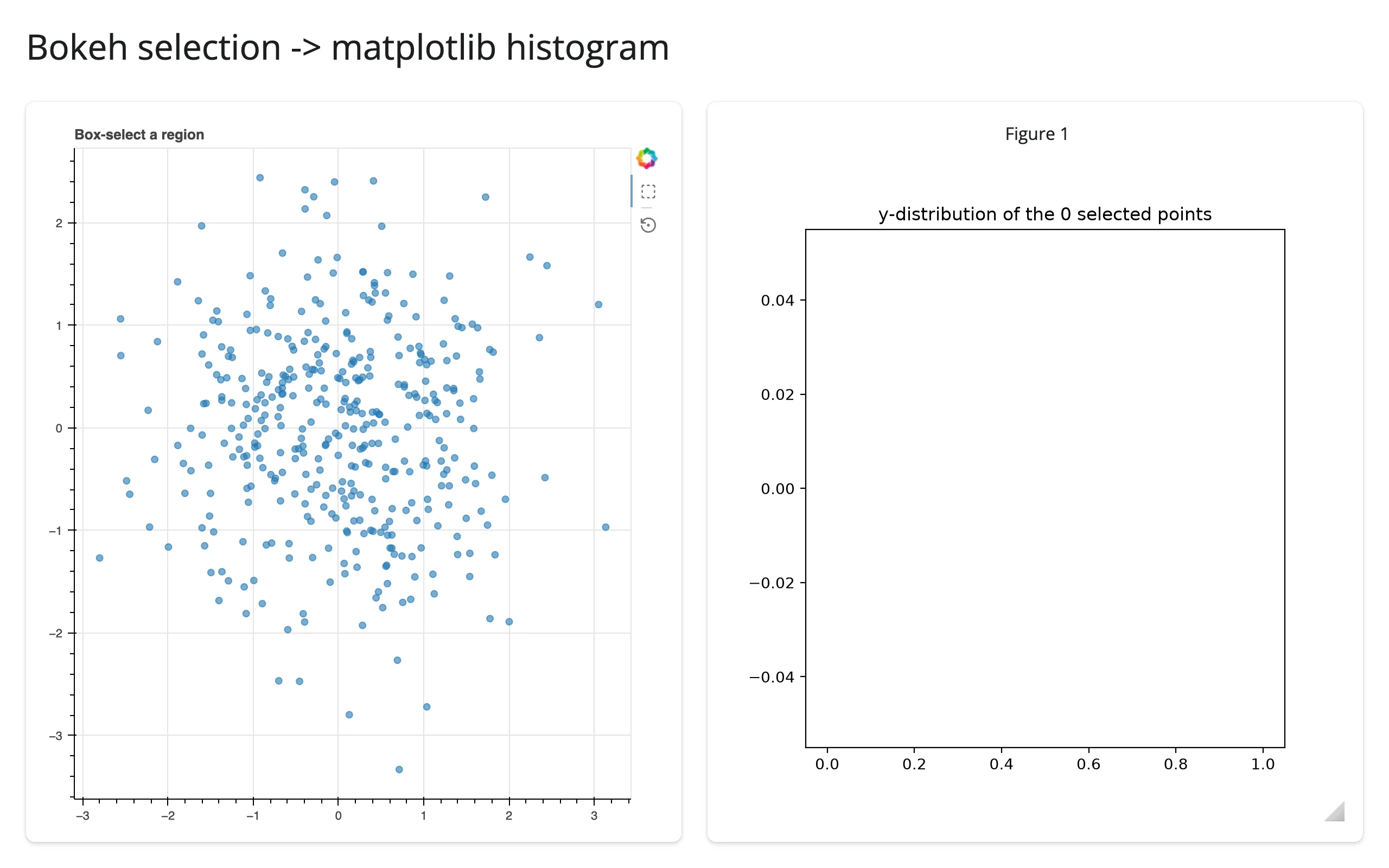

Tap for details

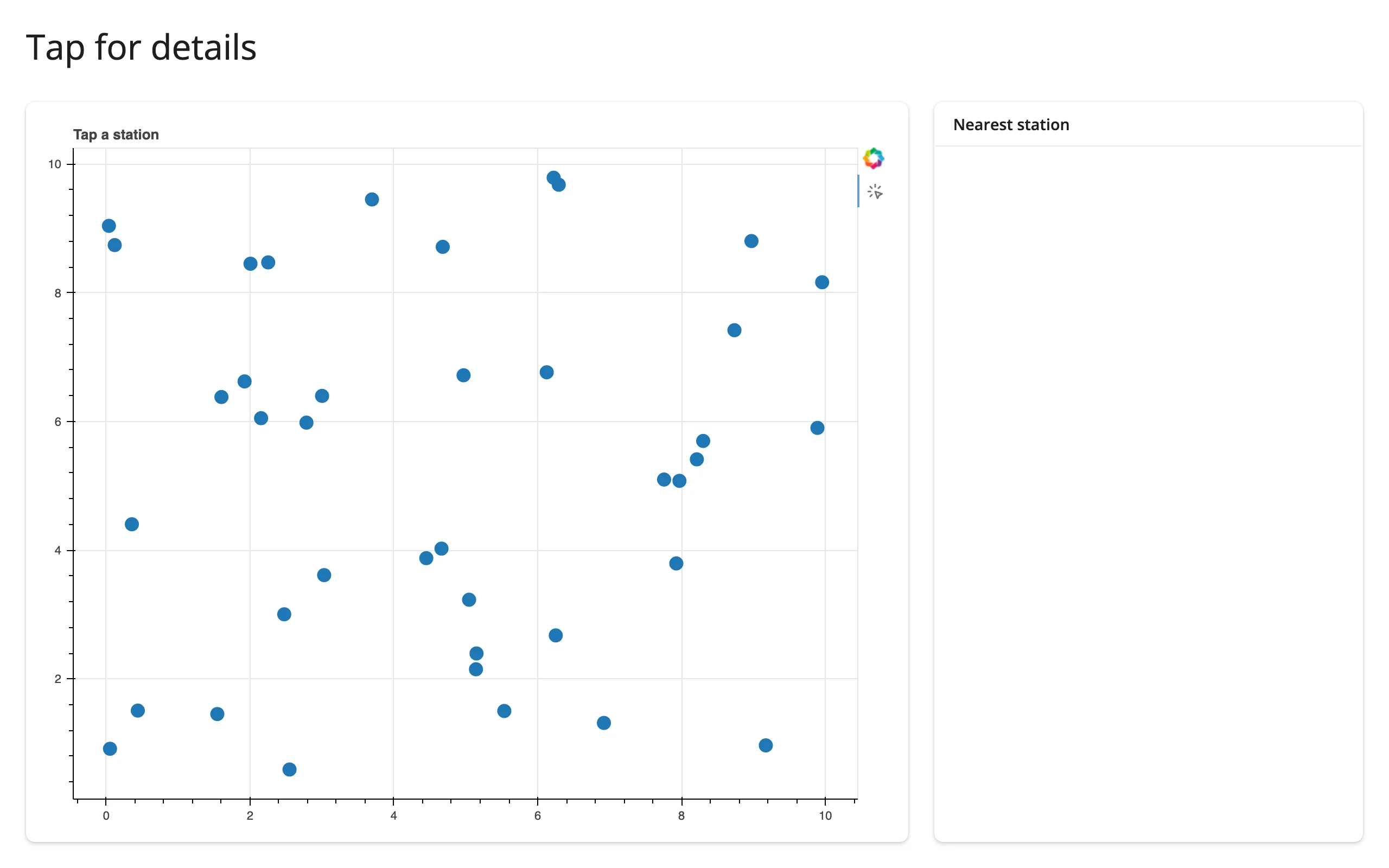
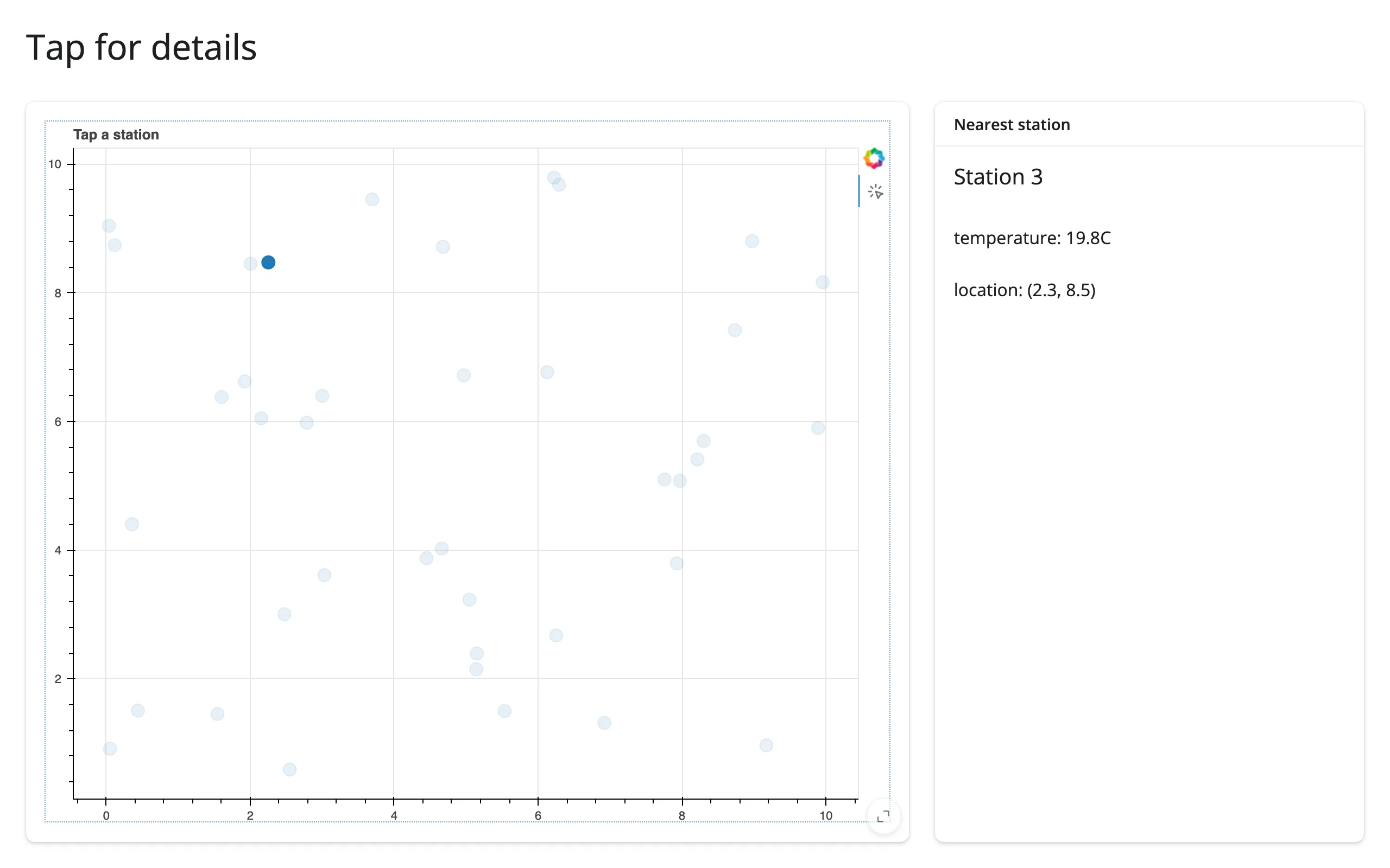
tapped() gives you a click location in data units, not necessarily a row – so look up the nearest point yourself. That’s more flexible than an auto-selecting tap tool: here it drives a detail card from a tap anywhere near a station:

examples/16_tap_to_detail.py42 lines

import numpy as np
from bokeh.models import ColumnDataSource
from bokeh.plotting import figure
from shiny import req
from shiny.express import render, ui
from shinywidgets import render_bokeh

ui.page_opts(title="Tap for details", fillable=True)

rng = np.random.default_rng(7)
n = 40
src = ColumnDataSource(
    {
        "x": rng.uniform(0, 10, n),
        "y": rng.uniform(0, 10, n),
        "city": [f"Station {i}" for i in range(n)],
        "temp": rng.normal(18, 5, n),
    }
)

with ui.layout_columns(col_widths=[8, 4]):
    with ui.card(full_screen=True):

        @render_bokeh
        def plot():
            p = figure(tools="tap", title="Tap a station")
            p.scatter("x", "y", source=src, size=12)
            return p

    with ui.card():
        ui.card_header("Nearest station")

        @render.ui
        def detail():
            t = req(plot.tapped())
            x, y = np.asarray(src.data["x"]), np.asarray(src.data["y"])
            i = int(np.argmin((x - t.x) ** 2 + (y - t.y) ** 2))
            return ui.TagList(
                ui.h5(src.data["city"][i]),
                ui.p(f"temperature: {src.data['temp'][i]:.1f}C"),
                ui.p(f"location: ({x[i]:.1f}, {y[i]:.1f})"),
            )

tap to detail before tap to detail after

Large data

figure(output_backend="webgl") draws glyphs on the GPU instead of the default HTML canvas 2D context. It’s a rendering-only switch: the two backends ship the same ColumnDataSource data over the websocket. Measured directly at 200,000 points, the two panels below sent effectively identical payloads (about 4.13 MB each, a 0.001% difference) – the same bytes either way, so output_backend="webgl" is purely about keeping pan/zoom smooth once the canvas backend starts to drop frames, not a way to shrink what crosses the wire:

examples/18_webgl_vs_canvas.py30 lines

import numpy as np
from bokeh.plotting import figure
from shiny.express import ui
from shinywidgets import render_bokeh

rng = np.random.default_rng(0)
n = 200_000
x = rng.normal(size=n)
y = x * 0.5 + rng.normal(size=n)

ui.page_opts(title="WebGL vs. canvas at 200,000 points", fillable=True)

with ui.layout_columns():
    with ui.card(full_screen=True):
        ui.card_header('output_backend="webgl"')

        @render_bokeh
        def webgl_plot():
            p = figure(output_backend="webgl", title="WebGL")
            p.scatter(x, y, size=3, alpha=0.3)
            return p

    with ui.card(full_screen=True):
        ui.card_header("default (canvas)")

        @render_bokeh
        def canvas_plot():
            p = figure(title="Canvas")
            p.scatter(x, y, size=3, alpha=0.3)
            return p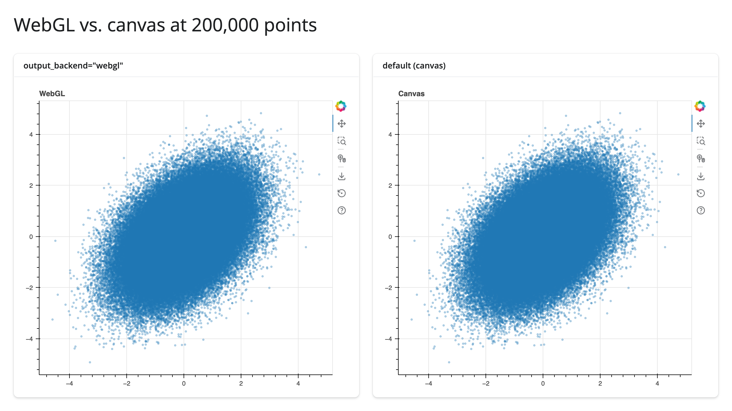

Time to first render also favors WebGL at this scale, not just steady-state pan/zoom smoothness: measured with isolated single-panel copies of the two apps above (three runs each, median reported), the WebGL panel reached a stable, fully-drawn scatter in 5.1 s versus 7.4 s for the canvas panel – about 30% faster, even though both ship the identical bytes measured above. Method and raw numbers in NOTES.md.

This is the “draw it with the GPU in the browser” approach from Large data & performance. For data that doesn’t fit even on the GPU as raw points, see datashader (which renders through @render_holoviews/Bokeh) to summarize server-side instead.

Layout and sizing

A bare figure() fills its output; giving it width, height, sizing_mode, or aspect_ratio opts out, and Bokeh’s own sizing applies instead (verified: the output’s fill only stays on when the figure’s sizing_mode is one of stretch_both/stretch_height/scale_both/scale_height).
For a layout (row, column, gridplot), set sizing_mode="stretch_both" on both the layout and each child figure. Setting it only on the outer layout (not the children) leaves the children at Bokeh’s own default size, and the layout’s flex box then divides space unevenly between them rather than splitting it evenly – examples/11_multiple_sources.py sets it on all three for this reason.
output_widget() (Shiny Core) or a plain @render_bokeh function under ui.card() (Express) is the same for Bokeh as for every other renderer; nothing Bokeh-specific to add.
bokeh_dependency() is deprecated and unnecessary – BokehJS loads automatically with every Bokeh-based output, including ones created dynamically inside @render.ui.

Gotchas and limitations

One ColumnDataSource per plot for selected()/selected_rows(). More than one raises TypeError; use each source’s own on_change("indices", ...) instead (see Several ColumnDataSources).
Plots that share a source must come from one render function. A ColumnDataSource (and any Bokeh model) can belong to only one Bokeh document; splitting linked plots across two @render_bokeh outputs fails with Bokeh’s own “Models must be owned by only a single document” error.
Build Bokeh models per session. In Shiny Express, top-level code already runs once per session, so this is automatic. In Shiny Core, construct figures and sources inside server() (or the render function) – a module-level figure is shared by every visitor, selections included.
Raw on_change/on_event callbacks fire twice per browser-driven change. Verified directly: a single box-select gesture called a hand-written source.selected.on_change("indices", ...) callback twice (confirmed with a counter). selected(), selected_rows(), tapped(), and zoomed() already dedupe this for you (one value per gesture); if you write your own raw callback instead (as in the Bokeh-widgets and draw-tool examples above), make it idempotent – setting a reactive.value already is, incrementing a counter isn’t.
Accessors can’t be read inside their own output’s render function. plot.selected() inside plot’s own @render_bokeh function raises RuntimeError – read it from another output or a @reactive.effect, and update the plot in place from there (see Updating the widget from Python).

Gallery candidates

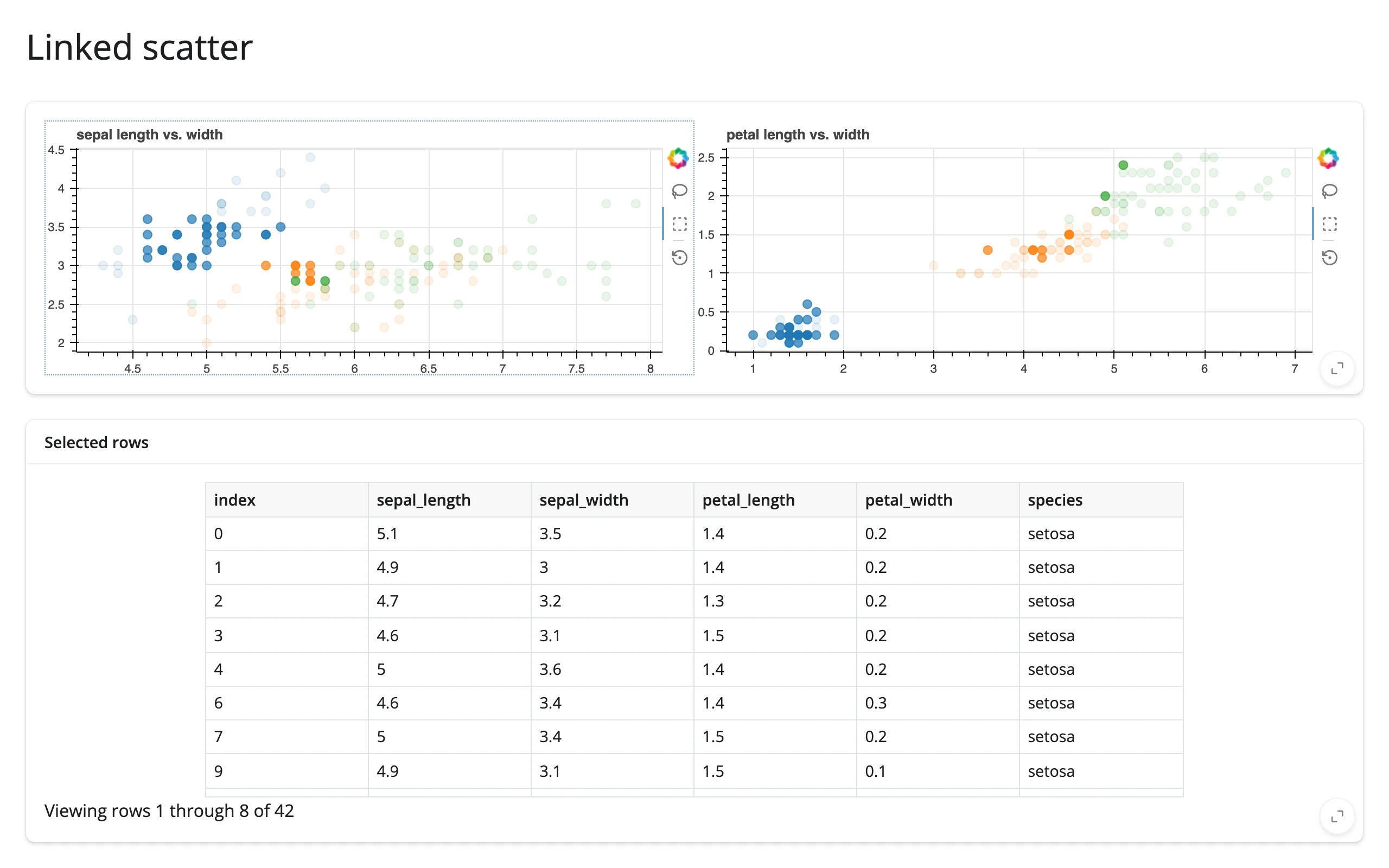
gallery/template_linked_scatter.py – two linked scatter plots over Fisher’s iris flowers (sepal and petal dimensions, colored by species) feeding a selected-rows table. A clean starting point for any 2-3-feature linked-brushing dashboard.

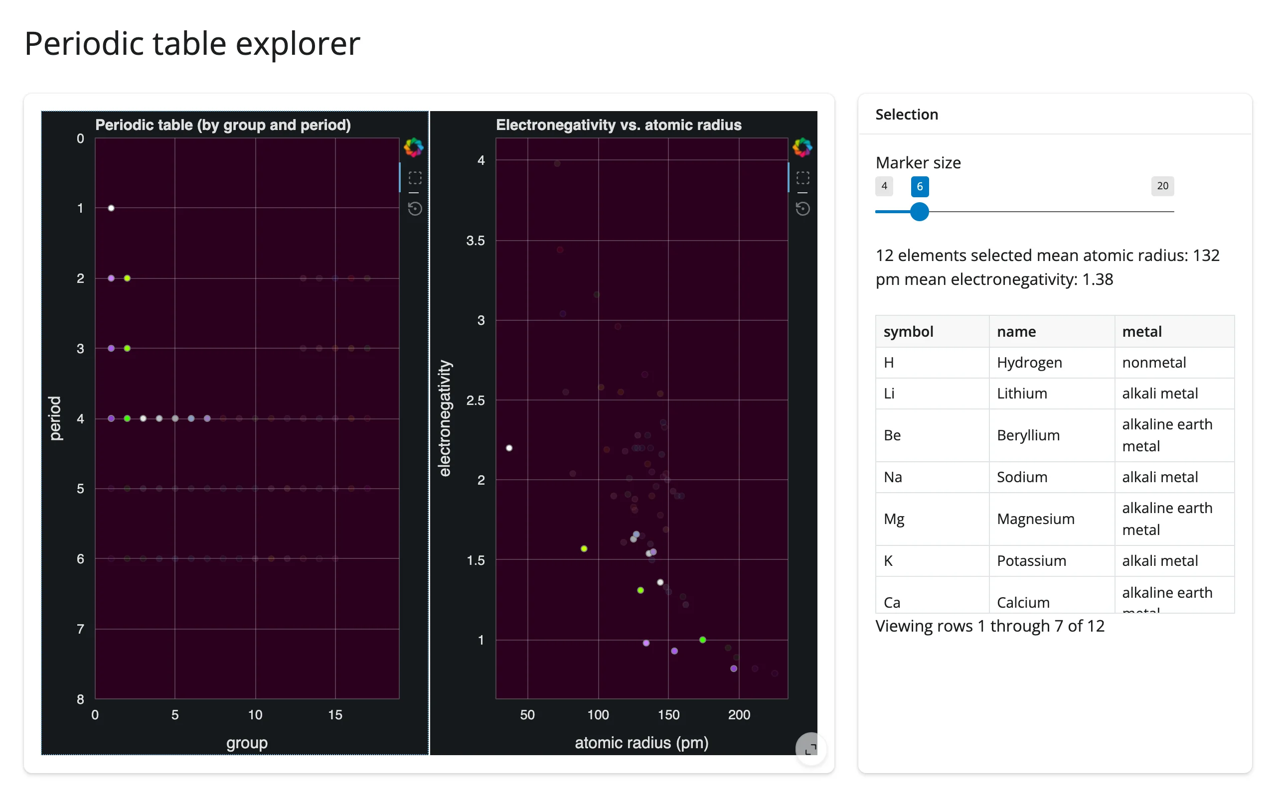
gallery/showcase_periodic_table.py – the periodic table grid linked to an electronegativity-vs-atomic-radius scatter, both colored with each element’s real CPK color on a dark theme. Box-select in either plot highlights the same elements in the other; a slider rescales markers in place by atomic mass.

Learn more

Bokeh user guide and reference
jupyter_bokeh, the bridge @render_bokeh builds on
Related guides in this roster: holoviews and panel, both of which render through Bokeh but don’t get accessors; plotly and altair for alternative plotting approaches; matplotlib, used above as the target of a cross-widget selection.