Choosing a widget

A by-task guide to the roughly 40 widget libraries shinywidgets integrates: which one to reach for selection/brushing, tables, maps, big data, 3D and scientific visualization, networks, drawing input, embedding exploration, and the “bring your own widget” escape hatch – with the trade-offs that actually matter in Shiny (accessors, in-place updates, measured scale, first-load cost, and maturity).

shinywidgets integrates roughly 40 widget libraries. Almost none of them compete head-to-head – each earns its place in the roster by doing one task well: GPU scatter plots at a scale DOM-based charts choke on, a full desktop-GIS map embedded in a Shiny card, a neuroimaging viewer, a molecule grid. The hard part isn’t learning any one of them (each has its own guide for that); it’s knowing which one to reach for, and when the honest answer is “you don’t need a widget at all – render.plot or render.data_frame already does this.”

This article is organized by task, not by library. For each task it names a default recommendation, the real trade-offs (not a feature-matrix dump), and links to the guide that goes deep on each candidate. Reacting to widgets explains what a reactive accessor is and how to read one; this release’s headline feature is that most of the plotting, table, and map widgets below now have them, so a user’s click, lasso, or drag flows back into Python as a normal reactive value, no JavaScript required. Linking widgets covers the shapes of apps you build once you’ve picked your widgets. This article answers the question one level up: which widgets.

three selection accessors, one gesture each: plotly’s dashed box, altair’s gray brush, bokeh’s highlighted points

How to read the trade-offs

Four things matter more in Shiny than they do in a notebook, because a Shiny app is long-running, multi-user, and server-rendered:

Accessors. Does user interaction (click, lasso, pan, edit) come back to Python as a named accessor you can read with req(), or do you have to fall back to .read("trait") (every renderer output has this, even with zero named accessors), or reactive_read() on a nested widget the output doesn’t wrap directly? More accessors generally means less code for you to write, but it only matters if your app needs that interaction. See Reacting to widgets for the three tiers.
In-place updates. Can you change the widget via .widget.<trait> = ... inside an effect (preserving zoom, camera, selection, and avoiding re-sending the JS bundle), or does every data change force a full re-render? This is the difference between an app that feels instant and one that flickers on every input change.
Scale. The point at which a widget stops being usable – measured by each guide, not guessed. A DOM-based table or map tops out in the thousands of rows; a GPU scatter plot or a server-side-aggregated raster keeps going into the millions or tens of millions.
Maturity and lifetime. Some integrations in this roster are new, upstream-fragile, or have a known fix sitting on an unmerged branch (see the callout boxes below). A few widgets also have real constraints on being shared across sessions (shared_lifetime()), which matters if you’re building a dashboard other people will use concurrently.

Statistical charts

Default: plotly, if you don’t already have a reason to pick something else. It has the richest accessor set in the whole roster – clicked(), double_clicked(), hover(), selected()/selecting(), brushed()/brushing(), relayout(), legend_clicked(), visible_traces(), and selected_rows() – covers click, double-click (a “view reset” pulse), hover, lasso/box select (both live-during-drag and settled), zoom/pan, and legend toggles, and plotly.express gets you a real chart in one line. See the plotly guide.

Reach for something else when:

You want the selection declared in the chart’s own grammar, not assembled from callbacks. Altair’s selected()/selected_rows() read a Vega-Lite selection_interval/selection_point you declare with .add_params(...) – the selection is part of the chart spec, which composes cleanly across layers and facets. Trade-off: two Vega-Lite selections sharing one view clear each other (a legend click clears a brush), and selected_rows() only matches layers using the identical underlying frame object.
You’re building Bokeh plots from live Python objects (a ColumnDataSource you mutate, a custom CustomJS), and want selected(), selected_rows(), tapped(), and zoomed() as accessors on top. See bokeh. One upstream quirk: raw on_change/on_event callbacks you register yourself fire twice per browser change (the accessors already dedupe this for you).
You need something already written in matplotlib or plotnine/ggplot2. render_matplotlib (clicked(), picked(), limits()) and render_plotnine (clicked(), limits(ax=0), same ipympl canvas) turn a static figure into a zoomable, clickable one without a rewrite – see matplotlib and plotnine. This is also the only path to a render.plot-style composition Shiny’s built-in static renderer can’t show at all (patchwork/subplot compositions).
You want grammar-of-graphics plots with native widget state (not just static output) and don’t mind a narrower community than Vega-Lite’s. bqplot’s selected()/brush() track per-mark selected indices and animate data updates in place; no clicked() by design (the figure’s own interaction overlay would swallow it).
You already live in HoloViews/hvPlot/Panel. Panel’s param(name) accessor (e.g., slider.param("value")) reads any rendered object’s param value reactively, no bridge code needed. HoloViews and obsplot still have no dedicated accessors – crossfilter via hv.link_selections, or read .read("trait")/reactive_read() on streams and params directly. See holoviews. One tip worth knowing up front: a composite hv.link_selections Layout (several linked elements) defaults to the Pan tool, not box-select, at any canvas width – set .opts(active_tools=["box_select"]) on each element so the box-select tool is armed without requiring a manual toolbar click first.

Use a plain render.plot instead when the chart is genuinely static (no zoom, no click, no data that changes after render) – a matplotlib figure doesn’t need render_matplotlib’s ipympl canvas, and you skip the bundle entirely.

Tables and grids: display vs. input

The question to ask first: does the user need to do anything with the table besides read it? If not, render.data_frame (plain Shiny core, no extra package) already gives you a virtualized, sortable grid with row selection via cell_selection() – no shinywidgets[...] extra, no bundle. Reach for a dedicated table widget only when you need one of these specific things it doesn’t have:

Need	Widget	Why
Zero-config global search, export (CSV/Excel), faceted SearchPanes filters	itables	`selected_rows()`; richest “classic DataTables” feature catalog of the three client-side tables
Rectangular cell-block selection, in-cell bars/heatmaps, editable cells	ipydatagrid	`selected()`, `clicked_cell()`, `edited_cell()`, `visible_data()` – the only one with real cell-block (not just row) selection
Grouping/aggregation, expandable detail rows, custom cell renderers, theming	reactable	richest display/theming feature set; `selected_rows()`, `page()`, `sorted()`, `filtered()`, `search()`
User-driven pivot/BI exploration: drag-and-drop group-by, a dozen chart plugins	perspective	`filter()`, `view_config()` round-trip the user’s own query as a dict
Browse millions of rows with per-column histograms, zero app code	quak	`sql()`/`data()`; a 5M-row table paints like 5k because only on-screen rows + histogram bins cross the wire – locked down by default, see callout below
Full Tableau-style ad hoc chart builder, size-independent cost	pygwalker	no accessors (only `on_msg` for save/export, plus the `.read()` tier for a bare trait); DuckDB computes every chart server-side, so 500 rows and 1,000,000 rows cost the same bytes and time
Several linked charts/tables/inputs crossfiltering one spec	mosaic	`params()`/`data(filter_by=...)`; the only dashboard-spec widget here, not a single view – locked down by default, see callout below

Security, quak and mosaic: both run browser-supplied SQL against the widget’s DuckDB connection, so an unrestricted connection would let a visitor read or write arbitrary server files. By default, the renderer locks the connection down before display (SET enable_external_access = false, SET lock_configuration = true) – the same pattern embedding-atlas uses. Pass allow_unrestricted_connection=True to opt out (e.g., a local, single-user app). For a shared DuckDB connection (con=, or a relation registered on duckdb.default_connection()), mosaic’s lockdown is permanent and database-wide – it also locks every other cursor on that connection, not just the widget’s – so do any server-side file reads before the first render, or opt out for that connection.

Maps and geospatial

Five different sub-tasks hide under “I need a map”:

Sub-task	Widget	Notes
Use the map itself as an input: draw a region, click a feature, read bounds/zoom	ipyleaflet	5 accessors (`bounds`, `zoom`, `center`, `clicked`, `drawn_features`) and a mature drawing toolbar; DOM-based, so prefer one GeoJSON layer over many `Marker`s past a few hundred points
One high-level API when you don’t know which engine you need	leafmap	a thin wrapper (`add_gdf`, `add_cog_layer`, split-map, legends, time sliders) over ipyleaflet, MapLibre, or kepler.gl – shares ipyleaflet’s 5 accessors on its default backend
Styled vector tiles, labels, 3D pitch/bearing/extrusion, globe projection	maplibre	real Mapbox GL style spec; comfortable to a few hundred thousand features; accessors `view_state()`, `clicked()`, `drawn_features()`; the migration target for deprecated pydeck
GPU scale: tens to hundreds of thousands of points, data-driven styling	lonboard	WebGL/deck.gl via GeoArrow (zero-copy, not GeoJSON); richest map selection model (`view_state`, `selected_index`, `selected_bounds`, `clicked`); the “scale” answer for everyone else in this list
Raster data: GeoTIFF/COG/elevation on a map, no separate tile service	localtileserver	produces an ordinary `ipyleaflet.TileLayer`; no accessors of its own (it’s a tile server, not a renderer); the only one engineered for safe deployment (per-session reverse proxy, guarded against path/SSRF abuse)
Real cartographic (non-Mercator) projections	geoviews	Cartopy projections through HoloViews/Bokeh; a server-side rasterization path (Datashader) for scaling past raw point rendering, same idempotent-subscriber caveat as holoviews
Hand the user a full desktop-GIS authoring app	geolibre	embeds the entire GeoLibre app (layer panel, styling, drawing, measuring) with two-way state sync; young and moves fast; blocking methods (`fly_to()`, `to_image()`) must run on a worker thread
Hand the user a no-code geospatial analysis studio	kepler.gl	auto-layers, filters, 3D hexbins, time playback, returns a reusable `config`; ships a ~12.9 MB JS bundle per fresh render, so in-place config updates matter more here than almost anywhere else in the roster

Upstream bug, lonboard: GlobeView permanently breaks view_state() sync (the browser sends pitch/bearing, which GlobeViewState has no fields for; the sync throws, silently, and never recovers). Stick to the default MapView if you need view_state() to keep working.

Deprecated: pydeck. render_pydeck is deprecated – pydeck >= 0.9 dropped its live Jupyter widget entirely, so no ipywidgets bridge can render a pydeck.Deck anymore. Bring your pdk.Layer objects to maplibre’s add_deck_layers() (works unchanged, recommended default) or re-express them in lonboard’s native API for very large data. See the pydeck migration guide.

Big data (10^5 - 10^7 points)

Three different strategies, not three competing widgets:

Render every point on the GPU. jscatter is the simplest version of this – a real WebGL scatter plot built for hundreds of thousands of points and up (the guide’s showcase runs 300k), with selected() giving you the lassoed row positions directly. No server aggregation, no SQL: every point really is in the browser. One upstream limit: only two of color/size/opacity can combine on one chart.
Aggregate on the server into a screen-sized image, and re-aggregate on every zoom. datashader (via render_holoviews) is built for the case where individual marks would be meaningless anyway – the payload is flat at about 6.9 MB whether you’re plotting 100k or 10M points (a plain scatter through the same renderer grows from 2.1 MB to 20.6 MB and doesn’t finish at 10M within 90 seconds), and re-aggregating after a wheel-zoom at 10M points took 0.24s measured. The cost: no true per-point picking, since a pixel can represent many points.
One widget, several linked views, crossfiltered through DuckDB. embedding-atlas packages a GPU map, auto-generated charts for every column, a searchable table, and SQL cross-filtering behind one predicate()/selected() accessor pair – built for thousands to millions of rows, at the cost of a hard WebGPU requirement for the map view itself (the rest still works without it). For tables specifically at this scale, see quak and mosaic above – same DuckDB-crossfilter idea, no map.

For point maps at this scale specifically, see lonboard in the next section.

3D and scientific visualization

This category is really ten different domains that happen to share “3D” as a label. Pick by domain, not by feature list:

Domain	Widget	Notes
Generic 3D scene: points, surfaces, isosurfaces, vectors	k3d	a do-everything scientific 3D plotter; 1M points stayed orbitable at interactive rates even on software rendering; `camera()` accessor plus click/hover picking callbacks
Volumetric (ray-marched) rendering	ipyvolume	the only widget here with real-time ray-marched `ipv.volshow()` and built-in frame animation; unmaintained upstream since 2021-2023 – don’t expect fixes, and a per-point string color array hangs the entire server process, not just the output
Arbitrary custom scene graph (meshes, lights, cameras you build by hand)	pythreejs	a direct three.js binding for when k3d/ipyvolume/pyvista’s higher-level APIs don’t cover what you need; several unfixed three.js-level upstream bugs (`mesh.rotation` is inert; lights leak browser objects per re-render)
Meshes/volumes/point clouds via VTK (CFD, geoscience, medical)	pyvista	the toolkit behind most scientific/medical 3D visualization; zero accessors by design – everything is re-render-driven, no camera/click ever reaches Python; current regression: a shared, process-wide viewer widget (trame-pyvista 0.3.x) breaks multi-session apps – fix exists on an unmerged branch, not yet on main
Molecular structures and MD trajectories	nglview	native trajectory playback (`.frame`, bidirectional with its own player) and atom-level click picking (`picked`, full residue/chain/element record)
Neuroimaging (NIfTI/DICOM volumes, overlays, surfaces)	niivue	clinical-grade WebGL2; the only widget with a true `location()` accessor (voxel/mm coordinates plus intensity under the crosshair); re-renders are expensive (~5 MB bundle plus the whole volume re-uploaded) – prefer in-place updates or `Volume(url=...)` for remote data
2D chemistry (SMILES, substructure search) – filed here despite the name	mols2grid	client-side RDKit WebAssembly powers SMARTS search; `selected()`/`clicked()` accessors; needs CDN access (fails silently, empty grid, if unreachable); tens of thousands of molecules approach the websocket message limit
Astronomy (real navigable sky, HiPS surveys)	ipyaladin	richest accessor set in this entire category (`clicked_object`, `selected_objects`, `target`, `fov`); needs live network access to CDS; `set_listener()` is a shared, cross-session-unsafe class-level dict – use the accessors instead in a multi-user app
Multimodal, time-indexed logs (3D + images + plots + text, one timeline)	rerun	streams live into an already-rendered viewer with no re-render; ~55 MB bundle by default (self-hostable); `rr.init()`’s default recording is process-global – use a per-session `RecordingStream` or one session’s data leaks into every other session’s viewer
Gigapixel multichannel bioimaging (OME-Zarr/OME-NGFF)	vizarr	multiscale pyramid tiling via Viv/deck.gl; no accessors, one synced `view_state` trait; pins `zarr<3`, which conflicts with vitessce’s `zarr>=3` – the two can’t share an environment
Single-cell / spatial-omics coordinated dashboards	vitessce	the entire interaction surface is one synced `_config` dict (every pan/zoom/lasso loops back); richest “coordinated multi-view dashboard in one output” story here, but the least mature: unreleased, only exists on an unmerged PR

The common thread across this whole category: most of these widgets have thin or no accessor surfaces compared to plotting/table widgets, because the interesting state (a VTK camera, a Vega-less 3D scene) often lives entirely client-side. When a widget here has no accessor you need, check its “Beyond the accessors: reactive_read” section before assuming the interaction is unreachable from Python.

Networks

Two widgets, and the choice is almost entirely about scale and styling depth, not features:

ipycytoscape for a themed, precisely styled graph – community/shortest-path coloring computed in Python with networkx, a CSS-like stylesheet, and a real layout vocabulary. Comfortable into the low thousands of nodes (every node and edge is its own ipywidgets model, so render time scales with element count). Lightly maintained upstream (last PyPI release in 2022); real open bugs worth knowing before you rely on them: removing a node from Python can corrupt the rest of the graph, and position/zoom/pan never sync browser to Python. clicked_node()/clicked_edge() (single click, kept across re-render) and selected_nodes()/selected_edges() (box/multi-select, debounced) accessors exist and work.
ipysigma for GPU-rendered scale – 20,000 nodes and 40,000 edges measured rendering promptly, with built-in search, legend filtering, and zoom/pan an SVG renderer can’t sustain. Trade-off: no named accessors (use the .read() tier for selected_node, selected_edge, camera_state, and friends), no Python-to-browser trait sync at all (changing a trait updates the model but nothing on screen until you re-render), and each Sigma view holds 3 WebGL contexts – browsers cap around 16 per page, so keep to about 5 ipysigma graphs on one page before older ones start going blank.

Drawing and canvas input

Three distinct “the user draws/picks something” tasks:

A hand-drawn dataset, for ML demos (classifier/regressor/clustering playgrounds, sculpting a distribution by hand): drawdata. The canvas output is a tabular dataset (points or bar heights), read via the .read() tier (data/brushsize) – no named accessors, but also no code needed to turn strokes into rows. One real limitation: BarWidget ignores every Python-side trait write after its first render, so it’s browser-driven only.
Arbitrary pixels, shapes, or a game loop: ipycanvas, a thin binding to the real HTML5 Canvas API – freehand sketch pads, pixel editors, cellular automata, click-to-annotate tools. No named accessors by design; wire raw mouse/keyboard callbacks to a reactive.value and read canvas.read("image_data") for the bitmap. Content is stateless per session (a refresh starts blank, no built-in undo).
A file already on the server’s filesystem: ipyfilechooser – the mirror image of Shiny’s own ui.input_file(), which uploads from the visitor’s machine. selected/selected_path are plain properties, not traits, so use register_callback() rather than reactive_read(). Sandbox it to a directory before pointing it at a multi-tenant server; unsandboxed, a visitor can browse anything the server process can read.

Use Shiny’s own ui.input_file() instead when you actually want the visitor to upload a file from their own machine – none of the three widgets above do that.

ML and embedding exploration

For exploring a set of embeddings (clusters, outliers, nearest neighbors), reach for embedding-atlas first – it was built for exactly this and gives you auto-generated per-column charts plus the map, all crossfiltered together. jscatter is the lighter-weight option if you already have a 2D projection and just want a fast, lassoable scatter plot without the rest of the workbench. For pairing either with an LLM-driven exploration loop (a chat interface that writes the filter/query for the user), see AI exploration.

Bring your own widget

If a third-party ipywidget, anywidget, or ipyreact widget you want isn’t in this roster at all (not every widget on PyPI gets a dedicated render_*), render_widget is the generic escape hatch: it renders any ipywidgets.Widget subclass, applies the same fill-sizing and as_widget() coercion the dedicated renderers get, and gives you .widget for in-place updates and .read("some_trait") for a reactive read (a shortcut for reactive_read() on .widget). It has no named accessors of its own and no library-specific bug fixes – always prefer a dedicated render_* when one exists in this roster, and fall back to render_widget only when one doesn’t.

A custom widget message (widget.send(), or a method like add_call()/add_basemap() that sends one under the hood) called from the render function itself, or from an effect that runs in the same flush as a re-render, is delivered once the widget’s comm opens, not dropped – a plain trait assignment always synced normally, and now a custom message does too. Some libraries’ own JavaScript still won’t visibly act on an early call until a later, genuine user gesture (browser autoplay-style restrictions, not a shinywidgets limitation) – see k3d’s Gotchas section for a worked example.

Comparison matrix

“Accessors” counts named reactive accessors on the renderer (0 means fall back to that output’s .read("trait") tier instead – not a dead end, just a different tier; see Reacting to widgets). “In-place” is whether you can update the rendered widget from an effect without a full re-render (preserving zoom/camera/selection). “Measured scale” is a number from the widget’s own guide, not a guess – “not benchmarked” means no guide measured a ceiling, not that one doesn’t exist.

Category	Widget	Accessors	In-place updates	Measured scale	Typical use
Charts	plotly	10	yes (`batch_update`)	WebGL past ~10k pts; 200k pts <1s	general-purpose interactive charting
Charts	altair	2	yes (`.widget.chart =`)	5,000-row cap unless VegaFusion/`disable_max_rows()`	grammar-of-graphics, native Vega-Lite selections
Charts	bokeh	4	yes (mutate `ColumnDataSource`)	not benchmarked	live Python object model, zero-round-trip linked views
Charts	matplotlib	3	yes (axes methods + redraw)	fine for typical use; use `render.plot` for very large data	make any existing matplotlib/seaborn/sklearn plot interactive
Charts	plotnine	2	no dedicated update API	exploration-sized	ggplot2-style plots, true plot compositions
Charts	bqplot	3	yes, tweened (`animation_duration`)	small-to-medium (fixed-pixel chrome)	charts that double as multi-point inputs
Charts	holoviews	0	yes (idempotent subscriber required)	not benchmarked	crossfilter dashboards via `link_selections`
Charts	datashader	0 (rides `render_holoviews`)	yes (flat payload)	flat ~6.9 MB payload at 100k/1M/10M points	aggregate 10M+ points server-side into an image
Charts	jscatter	2	see guide	hundreds of thousands and up (300k in showcase)	simplest huge GPU scatter plot with lasso
Charts	obsplot	0	yes (`.widget.spec =`)	message size grows with data; aggregate first	Observable Plot’s exact grammar and look
Charts	panel	1 (`param(name)`, dynamic)	yes (set the Panel object’s params, e.g. `.value =`)	not benchmarked	reuse Panel’s component library as one Shiny output
Tables & grids	itables	1	limited (`.update()` drops some options)	whole frame client-side; downsamples past 64KB JSON	zero-config searchable/sortable/exportable table
Tables & grids	reactable	5	yes (`props["data"]`)	not a big-data tool	grouping/aggregation, expandable rows, theming
Tables & grids	ipydatagrid	4	yes (`set_cell_value*`, `StreamingDataGrid`)	plain grid ships whole frame; `StreamingDataGrid` serves visible window only	rectangular cell-block selection, in-cell rendering, editing
Tables & grids	perspective	2	yes (`.update()`/`.clear()`; `.replace()` broken upstream)	strong through hundreds of thousands of rows (WASM)	user-driven pivot/BI exploration
Data exploration	pygwalker	0 (`on_msg` tier)	via `update_spec` on save	cost flat from 500 to 1,000,000 rows (DuckDB server-side)	full ad hoc Tableau-style chart builder
Data exploration	quak	2 (DuckDB locked down by default)	yes	5M-row table paints like 5k	browse millions of rows via per-column histograms, zero app code
Data exploration	mosaic	2 (DuckDB locked down by default)	yes (`.widget.spec =`)	1M rows brushed with no lag (raster/density marks never ship points)	several linked views crossfiltering one spec
Data exploration	embedding-atlas	2	yes	thousands to millions (map view needs WebGPU)	one-widget embedding workbench (map+charts+table+SQL)
Maps & geospatial	ipyleaflet	5	yes	DOM-based; prefer one GeoJSON layer past a few hundred markers	map as interactive input, per-layer control
Maps & geospatial	leafmap	5 (default backend)	yes (inherits backend)	inherits chosen backend	one high-level API across 3 map engines
Maps & geospatial	maplibre	3	yes (restyle in place, verified)	comfortable to a few hundred thousand features (140k demoed)	styled vector tiles, 3D/globe, deck.gl layers
Maps & geospatial	lonboard	5	yes (preserves zoom/camera)	tens/hundreds of thousands of GPU points, smooth	GPU map scale + data-driven styling
Maps & geospatial	geolibre	0	yes (two-way project-state sync)	not benchmarked (full app UI)	embedded desktop-GIS authoring app for end users
Maps & geospatial	kepler.gl	0	yes (matters more: ~12.9 MB bundle/render)	not benchmarked numerically this pass	no-code geospatial analysis studio, time playback
Maps & geospatial	geoviews	0	yes (idempotent subscriber required)	200k points demoed raw vs. rasterized	real cartographic projections + Datashader scale path
Maps & geospatial	localtileserver	0	yes (band/colormap/vmin-vmax restyle verified)	n/a – raster tile server, not a feature-count renderer	local/remote raster (GeoTIFF/COG) on a map
Maps & geospatial	pydeck (deprecated)	0	n/a	historically 140k points before breaking	none – migrate to maplibre or lonboard
3D	k3d	1	yes (gate behind user action)	1M points interactive, even on software rendering	generic do-everything scientific 3D scene
3D	pythreejs	1	yes	not a scale play (scene-graph flexibility)	arbitrary custom 3D scene graph
3D	pyvista	0	limited (snapshot-based)	payload ~proportional to mesh size (12 KB - 800 KB measured)	VTK meshes/volumes/point clouds (CFD, geoscience, medical)
3D	ipyvolume	1	yes	tens of thousands (GPU-instanced); unmaintained upstream	ray-marched volumetric rendering
Scientific	mols2grid	2	see guide	tens of thousands of molecules approach the websocket limit	2D chemistry grid, SMARTS substructure search
Scientific	nglview	0	yes (`.frame` bidirectional)	streams only changed atom coordinates per frame	molecular structures and MD trajectories
Scientific	vitessce	0	yes, 3 measured cost tiers (23-132 requests)	n/a (dashboard, not point-count)	single-cell/spatial-omics coordinated dashboards
Scientific	vizarr	0	limited (camera restore races deck.gl on re-render)	gigapixel via multiscale pyramids	gigapixel multichannel bioimaging (OME-Zarr)
Scientific	niivue	1	yes (preferred over re-render)	~5 MB bundle + full volume reupload per full render	neuroimaging (clinical-grade WebGL2)
Scientific	ipyaladin	4	yes (`target`/`fov` follow Python)	not a point-count story	real navigable sky atlas (astronomy)
Scientific	rerun	1	yes (streams live, no re-render)	built for continuous streaming, not a fixed ceiling	multimodal, time-indexed logs (robotics)
Networks	ipycytoscape	4	limited (zoom-from-Python has no effect)	comfortable into the low thousands of nodes	themed/styled graph, community/shortest-path coloring
Networks	ipysigma	0	no (no Python-to-browser trait sync at all)	20,000 nodes / 40,000 edges verified	GPU network explorer for large graphs
Input & drawing	drawdata	0	no (`BarWidget` ignores post-render writes)	n/a (small hand-drawn datasets)	freehand dataset drawing for ML demos
Input & drawing	ipycanvas	0	yes (draw commands; content is stateless per session)	thousands of shapes, or a full-res image, quickly	raw canvas drawing/game-loop input
Input & drawing	ipyfilechooser	0	n/a	n/a	server-side file picker (sandboxed)
Concepts	render_widget	0	yes	n/a – depends entirely on the wrapped widget	escape hatch for any ipywidget/anywidget without a dedicated guide

Decision flow

Start here if you’d rather answer a question than read a table.

Need selection/click events back in Python, from a chart? → Already using plotly, altair, or bokeh? Stay there – all three have accessors (plotly’s set is richest). → Starting from scratch and it’s a 2D scatter plot? plotly for the most accessor coverage, altair if you want the selection declared in the chart’s own grammar. → Hundreds of thousands of points or more? jscatter.

Need selection/click events back in Python, from a map? → Few hundred features, need draw tools or per-layer control? ipyleaflet. → Tens of thousands to millions of points? lonboard. → No accessors needed, just a styled basemap with 3D/globe? maplibre.

Just need to show a table, nothing more? → render.data_frame (Shiny core, no extra package). Add a widget only once you need search + export (itables), rectangular cell editing (ipydatagrid), or pivoting (perspective).

Data too big to put a mark on screen per row (>~500k rows)? → A table? quak or mosaic (DuckDB crossfilter). → A scatter plot? datashader (server-side rasterized) or jscatter (real GPU points, no aggregation). → A map? lonboard. → An exploratory workbench over all of the above at once? embedding-atlas (needs WebGPU).

3D, and you know which domain? → Generic scene: k3d. → VTK mesh/volume you already have in pyvista: pyvista (mind the multi-session caveat above). → Molecule/protein: nglview (structures) or mols2grid (2D SMILES grids). → Brain/medical volume: niivue. → Sky survey: ipyaladin. → Microscopy image pyramid: vizarr. → Single-cell/spatial-omics dashboard: vitessce (not yet merged). → Robotics/multimodal log stream: rerun.

A graph/network? → Thousands of nodes, want fine styling control: ipycytoscape. → Tens of thousands of nodes, want it to stay smooth: ipysigma.

The user needs to draw or pick something by hand? → A dataset to feed a model: drawdata. → Arbitrary pixels/shapes/a game loop: ipycanvas. → A file already on the server: ipyfilechooser. → A file from the visitor’s own computer: plain ui.input_file(), no widget needed.

None of the above fits (a third-party ipywidget/anywidget without a dedicated guide)? → render_widget.

Examples

Three short apps, each showing the same task implemented in two or three different widgets, side by side, so the differences are visible rather than described.

Selection: plotly vs. altair vs. bokeh

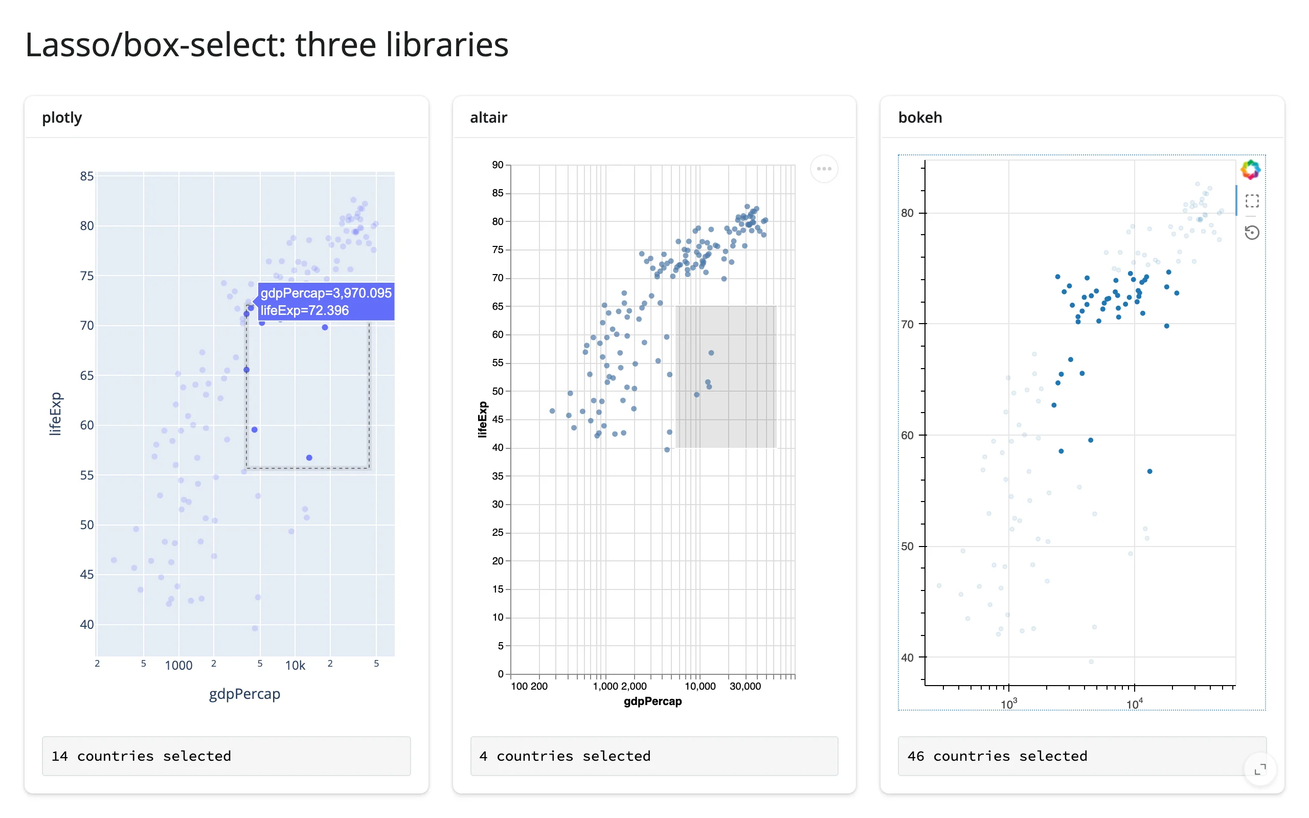
The same gapminder-2007 scatter plot (GDP per capita vs. life expectancy), box-selected in all three libraries. Same task, three different selection idioms: plotly’s dashed selection box, altair’s declared selection_interval (drawn as a gray brush), bokeh’s BoxSelectTool. All three report back through a selected_rows()-shaped accessor.

examples/01_selection_three_libraries.py64 lines

# Same lasso-selection task in plotly, altair, and bokeh, side by side.
# Shows how similar the *shape* of the task is across libraries, and the one
# real difference: altair's selection is declared in the chart spec (a
# grammar object you read by name); plotly's and bokeh's are accessors on
# the renderer itself, driven by `dragmode`/`BoxSelectTool`.
# Run: uv run shiny run docs/widget-guides/articles/choosing-a-widget/examples/01_selection_three_libraries.py
import altair as alt
import plotly.express as px
from bokeh.models import ColumnDataSource
from bokeh.plotting import figure
from shiny.express import render, ui
from shinywidgets import render_altair, render_bokeh, render_plotly

ui.page_opts(title="Lasso/box-select: three libraries", fillable=True)

df = px.data.gapminder().query("year == 2007").reset_index(drop=True)

with ui.layout_columns():
    with ui.card(full_screen=True):
        ui.card_header("plotly")

        @render_plotly
        def plot_plotly():
            fig = px.scatter(df, x="gdpPercap", y="lifeExp", log_x=True, custom_data=[df.index])
            fig.update_layout(dragmode="select", margin=dict(l=16, r=16, t=16, b=16))
            return fig

        @render.code
        def count_plotly():
            rows = plot_plotly.selected_rows(df)
            return f"{len(rows)} countries selected"

    with ui.card(full_screen=True):
        ui.card_header("altair")

        @render_altair
        def plot_altair():
            brush = alt.selection_interval(name="brush")
            return (
                alt.Chart(df)
                .mark_circle()
                .encode(x=alt.X("gdpPercap", scale=alt.Scale(type="log")), y="lifeExp")
                .add_params(brush)
            )

        @render.code
        def count_altair():
            rows = plot_altair.selected_rows("brush")
            return f"{len(rows)} countries selected"

    with ui.card(full_screen=True):
        ui.card_header("bokeh")

        @render_bokeh
        def plot_bokeh():
            source = ColumnDataSource(df)
            fig = figure(x_axis_type="log", tools="box_select,reset", active_drag="box_select")
            fig.scatter("gdpPercap", "lifeExp", source=source)
            return fig

        @render.code
        def count_bokeh():
            rows = plot_bokeh.selected_rows()
            return f"{len(rows)} countries selected"

Before and after a real box-select drag on all three panels:

before: three identical unselected scatter plots after: plotly’s dashed selection box (14 selected), altair’s gray brush (4 selected), bokeh’s highlighted points (46 selected)

The counts differ because each library’s own axis scaling puts the drag box over a different data range – not a bug. The point is the shape of the code: plotly and bokeh read an accessor on the renderer; altair reads an accessor keyed by the selection’s name, because in Vega-Lite the selection is part of the chart spec, not an afterthought bolted onto the renderer.

Tables: plain Shiny vs. itables vs. ipydatagrid

The same 142-country data frame through three outputs. render.data_frame needs no extra package and already supports row selection and per-column filters. itables adds a global search box and a one-line CSV export button. ipydatagrid adds rectangular, multi-cell selection (not just rows).

examples/02_tables_display_vs_input.py56 lines

# The same data frame through three table outputs, to show what each adds
# over plain Shiny: render.data_frame (free, built in, virtualized), itables
# (global search, export, zero config), ipydatagrid (cell-block selection,
# editable cells). None of these needs the others -- pick by what the task
# needs, not by default.
# Run: uv run shiny run docs/widget-guides/articles/choosing-a-widget/examples/02_tables_display_vs_input.py
import plotly.express as px
from ipydatagrid import DataGrid
from itables.widget import ITable
from shiny import req
from shiny.express import render, ui
from shinywidgets import render_ipydatagrid, render_itables

ui.page_opts(title="Tables: plain Shiny vs. itables vs. ipydatagrid", fillable=True)

df = px.data.gapminder().query("year == 2007").reset_index(drop=True)
cols = ["country", "continent", "lifeExp", "gdpPercap", "pop"]

with ui.layout_columns():
    with ui.card(full_screen=True):
        ui.card_header("render.data_frame -- plain Shiny, no extra JS")

        @render.data_frame
        def grid_plain():
            return render.DataGrid(df[cols], selection_mode="row", filters=True)

        @render.code
        def sel_plain():
            idx = grid_plain.cell_selection()["rows"]
            return f"{len(idx)} row(s) selected (click a row)"

    with ui.card(full_screen=True):
        ui.card_header("itables -- global search + export, built in")

        @render_itables
        def table_itables():
            return ITable(df[cols], select=True, buttons=["csvHtml5"])

        @render.code
        def sel_itables():
            n = len(table_itables.selected_rows())
            return f"{n} row(s) selected (click to search/select)"

    with ui.card(full_screen=True):
        ui.card_header("ipydatagrid -- rectangular cell-block selection")

        @render_ipydatagrid
        def grid_datagrid():
            return DataGrid(df[cols], selection_mode="cell")

        @render.code
        def sel_datagrid():
            blocks = req(grid_datagrid.selected())
            r1, r2 = blocks[0]["r1"], blocks[0]["r2"]
            c1, c2 = blocks[0]["c1"], blocks[0]["c2"]
            return f"block: rows {r1}-{r2}, cols {c1}-{c2} (click, then shift-click)"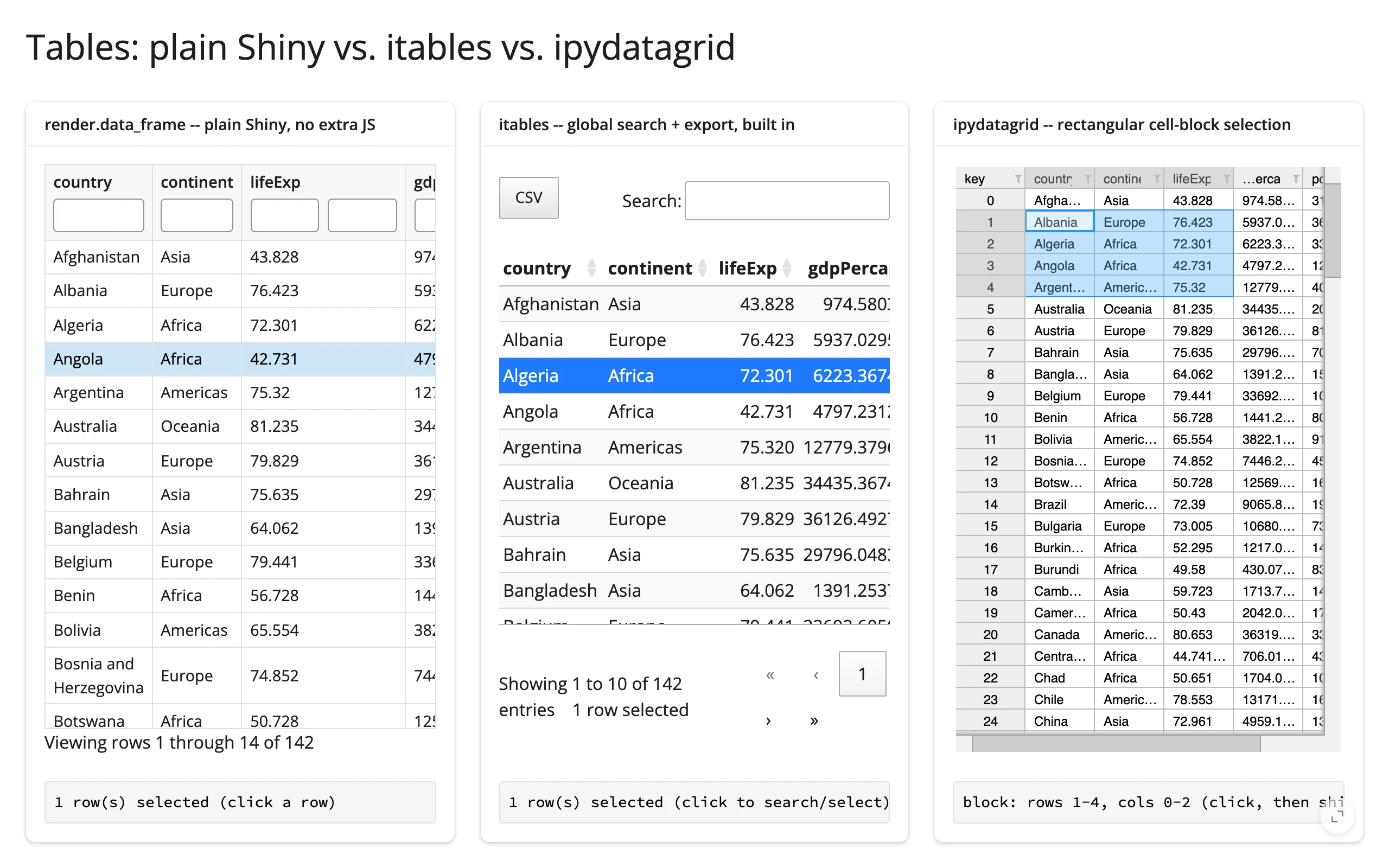

all three tables after a row click, a search-box row click, and a shift-click cell block

Maps: a location click vs. a feature pick

The same 249 real car2go pod locations around Montreal, in ipyleaflet (every point a real DOM marker) and lonboard (one GPU ScatterplotLayer). The API difference is the point: ipyleaflet’s clicked() reports where you clicked ({"coordinates": [lat, lng]}) and your code finds the nearest feature; lonboard’s selected() reports which row you picked directly, because deck.gl does GPU-native hit-testing. Neither is “better” – ipyleaflet gives you per-layer control (clustering, popups, draw tools) that a GPU layer doesn’t; lonboard’s picking is exact and scales to far more points than 249 (see Big data, above, and the lonboard guide for the hundred-thousand-point case).

examples/03_maps_location_vs_feature_pick.py59 lines

# The same "click a point, see its detail" task on the same 249 real
# car2go pods (Montreal), in ipyleaflet and lonboard. The point: ipyleaflet's
# clicked() reports a *location* (you find the nearest feature yourself);
# lonboard's selected() reports the picked *row* directly. Neither is
# "better" -- ipyleaflet gives per-layer control (clustering, popups,
# drawing); lonboard gives GPU-native picking that also scales past the ~250
# points shown here (see the lonboard guide for the multi-hundred-thousand-
# point case).
# Run: uv run shiny run docs/widget-guides/articles/choosing-a-widget/examples/03_maps_location_vs_feature_pick.py
import geopandas as gpd
import ipyleaflet as L
import plotly.express as px
from lonboard import Map as LonboardMap
from lonboard import ScatterplotLayer
from shiny import req
from shiny.express import render, ui
from shinywidgets import render_ipyleaflet, render_lonboard

ui.page_opts(title="Click-to-detail: ipyleaflet vs. lonboard", fillable=True)

pods = px.data.carshare()  # 249 real car2go pod locations around Montreal

with ui.layout_columns():
    with ui.card(full_screen=True):
        ui.card_header("ipyleaflet: clicked() is a location")

        @render_ipyleaflet
        def map_leaflet():
            m = L.Map(center=(45.52, -73.59), zoom=11)
            markers = [L.CircleMarker(location=(r.centroid_lat, r.centroid_lon), radius=4) for r in pods.itertuples()]
            m.add(L.LayerGroup(layers=markers))
            return m

        @render.ui
        def detail_leaflet():
            c = req(map_leaflet.clicked())
            lat, lng = c["coordinates"]
            d2 = (pods["centroid_lat"] - lat) ** 2 + (pods["centroid_lon"] - lng) ** 2
            row = pods.loc[d2.idxmin()]
            return ui.div(f"Nearest pod #{row.name}: {row['car_hours']:.0f} car-hours")

    with ui.card(full_screen=True):
        ui.card_header("lonboard: selected() is the row")

        @render_lonboard
        def map_lonboard():
            gdf = gpd.GeoDataFrame(
                pods, geometry=gpd.points_from_xy(pods.centroid_lon, pods.centroid_lat)
            )
            layer = ScatterplotLayer.from_geopandas(
                gdf, get_fill_color=[255, 60, 120], radius_min_pixels=5, pickable=True
            )
            return LonboardMap(layer, show_side_panel=False)

        @render.ui
        def detail_lonboard():
            index = req(map_lonboard.selected())
            row = pods.iloc[index]
            return ui.div(f"Picked pod #{row.name}: {row['car_hours']:.0f} car-hours")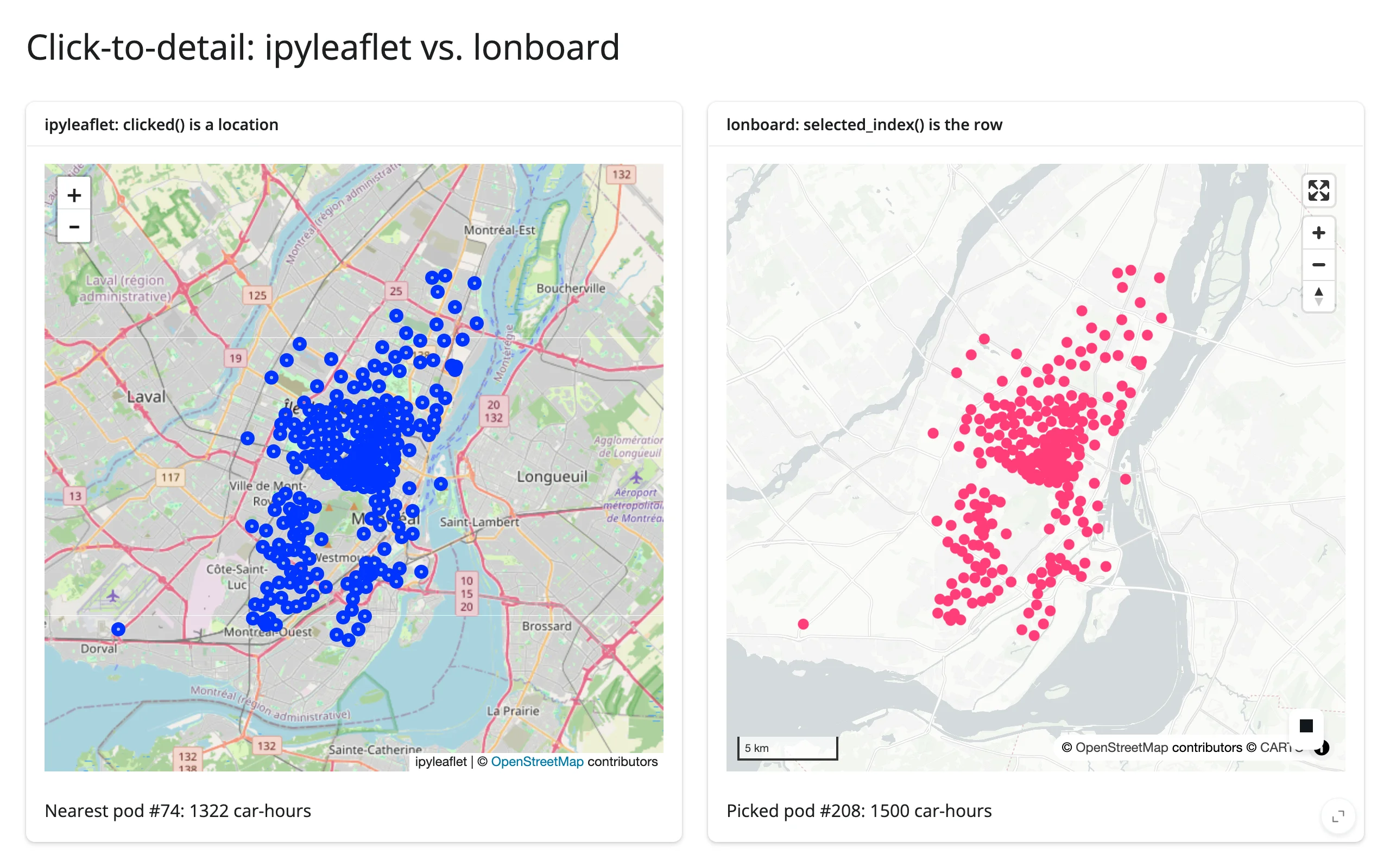

ipyleaflet shows the nearest pod to a blank-area click; lonboard shows the exact picked pod

Gotcha: the two clicked() accessors aren’t shaped the same. ipyleaflet returns a dict, {"coordinates": [lat, lng]} (latitude first). lonboard returns a bare tuple, (lng, lat) (longitude first). Mixing the two up silently swaps your latitude and longitude. Keep this guide open the first time you port code from one to the other.

Learn more

Reacting to widgets – what an accessor is, None semantics, rate policies, reactive_read(), in-place updates, widget lifetimes.
Linking widgets – the shapes of apps built from these accessors (selection to table, map to chart, table to plot, crossfilter, bidirectional linking).
Every widget named above has its own guide at ../../<slug>/guide.md with the full accessor reference, verified code, and a Gotchas section.